To remove the percentage from your data in Microsoft Excel, select the data, navigate to the Home tab, click the small arrow beside the Number format, and choose General for the format style.
In this article, you’ll learn a variety of ways to remove percentages from numbers in your data. It can take just a few seconds if you follow one of the methods below!
Quick Jump
ToggleMethod 1: Using the Home Tab
Difficulty: Beginner
Time Estimate: 5 Seconds
1. Select your data (A1:A5).
2. Go to the Home tab.
3. Click on the small arrow beside the Number format.
4. Pick the General option.
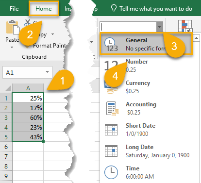
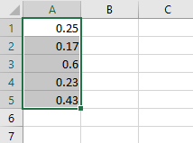
And there you go! The percentages have been removed.
Method 2: Using Custom Formatting
Difficulty: Beginner
Time Estimate: 15 Seconds
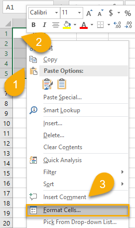
1. Select the data written as a percentage (A1:A5).
2. Right-click on the selected values.
3. Pick Format Cells.
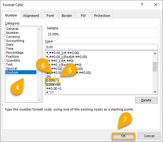
4. Choose the Custom category.
5. Select 0.00% as the type.
6. Press Ctrl+J between 0.00 and %.
7. Click OK.
8. Again select your data (A1:A5).
9. Navigate to the Home menu.
10. Click on the Wrap Text option.
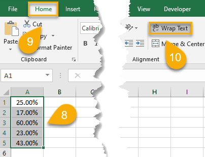
Easy as ABC! You have successfully removed the percentage.
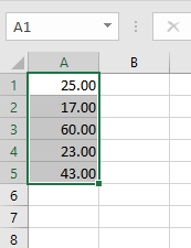
Method 3: Using Formulas
Difficulty: Beginner
Time Estimate: 15 Seconds
1. Click on the cell where you need to get the result.
2. Go to the Formula bar and type =VALUE(LEFT(TEXT(A1,”000.0000%”), 25)), where A1 is the cell with your percentage value, and 25 is the number from which you want to remove the percentage.
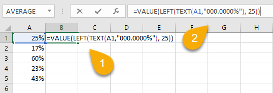
3. Press the Enter key on your keyboard.
4. Drag the cell downward to copy the formula for the rest of the list.
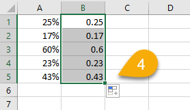
Voila! Let’s move on.
Method 4: Using VBA
Difficulty: Beginner
Time Estimate: 40 Seconds
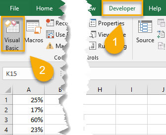
1. Go to the Developer tab.
2. Pick the Visual Basic option.
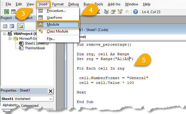
3. Click Insert.
4. Choose the Module option.
5. Enter the following code:
Sub remove_percentage()
Dim rng, cell As Range
Set rng = Range(“A1:A5”)
For Each cell In rng
cell.NumberFormat = “General”
cell = cell.Value * 100
Next
End Sub
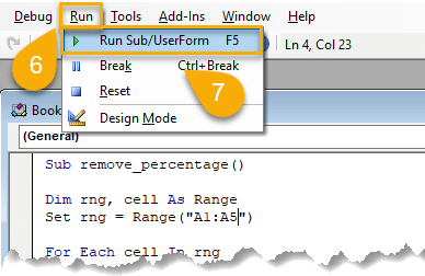
6. Click the Run tab.
7. Tap the Run Sub/UserForm option.
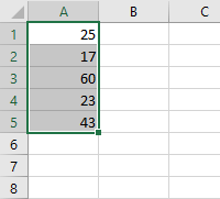
Piece of cake!
Method 5: Using Power Query
Difficulty: Beginner
Time Estimate: 1 Minute
1. Navigate to the Data tab.
2. Click From Table/Range.
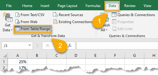
3. Set the range (the cells with your data).
4. Hit OK.
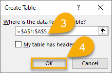
5. Click on the Add Column menu.
6. Select Custom Column.
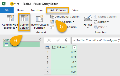
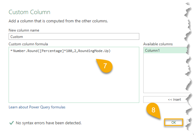
7. Enter the formula =Number.Round([Percentage]*100,2,RoundingMode.Up) in the Formula box.
8. Click OK.
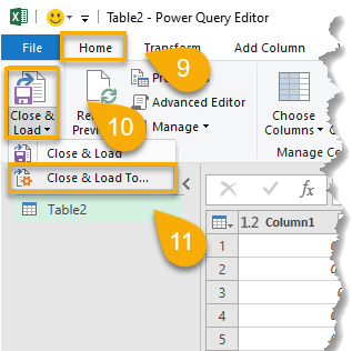
9. Go to the Home tab.
10. Choose Close & Load.
11. Pick Close & Load To from the list.
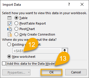
12. Choose the location where you want to import the data.
13. Click OK.
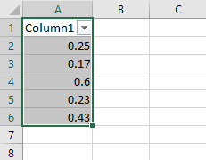
That’s it! You have done it!
Percentage FAQs
We suggest reading through the questions and answers below to better grasp this subject.
Why are percentages important?
Percentages are important because they help you understand the data that you are working with. They also help you see how much of a change there is in the data over time.
What are the rules for percentages?
To calculate a percentage, you first need to know the basic rules for percentages. A percent is simply a ratio or fraction with 100 as its denominator (base). So, if you have 50% of something, that means you have 50/100 or 1/2 of it. To find the percentage of something, you need to multiply the number by the decimal form of the percent (e.g., 70% = 0.70).
Why are percentages reversible?
As you probably know, percentages are a way to express a number as a part of 100. What you may not know is that this relationship is actually reversible: if you have the percentage, you can find the original number, and if you have the original number, you can find the percentage.