
Identifying deliverables and meeting deadlines is essential for completing a project within a specified timeframe. A burndown chart can help you evaluate a project’s workload and the time requirement for completing each task to determine proper scheduling.
A burndown chart is a superb tool for visualizing workload, and this article will provide a detailed step-by-step guide that will show you how to create one in Google Sheets.
What Is a Google Sheets Burndown Chart?
A burndown chart in Google Sheets is a graph that shows the progress of a project using four measures:
- The amount of time planned for work (planned hours)
- The actual amount of work done (actual output/hours)
- The amount of work left to do (remaining output/effort)
- The project’s overall estimated time of completion (ideal burndown)
With these four measures, you can use a burndown chart to understand how a project progresses in relation to its requirements.
It provides insight that helps you or your team identify how much time is needed to complete the project and how close or far away from the completion date the team is.
A burndown chart also allows you to evaluate your team’s level of efficiency and pinpoint the period when your team’s effort started to fall short of what was required.
There are two types of burndown charts: Product and Sprint burndown charts.
- A product burndown chart focuses on the entire project. It visualizes all project goals while providing insight into how much has been achieved.
- A sprint burndown chart focuses on only one specific aspect of the project. It visualizes a part of the project’s goals that a team sets out to achieve within a specific time.
How to Make a Burndown Chart in Google Sheets (Step-By-Step)
Let’s say your team was assigned four tasks to be completed in four weeks, with an estimated 80 hours to complete the tasks. At the end of the fourth week, your team didn’t meet the deadline.
To understand what went wrong, you proceed to create a burndown chart. Here’s how to begin.
Step 1: Prepare the Data
The first step to creating a burndown chart is to prepare the dataset. For a burndown chart, you need to set up two separate tables.
The first table details the historical information regarding the number of hours spent on each task.
Ideally, the original data will have columns for task categories, initial estimates, days/weeks/months, and remaining hours.
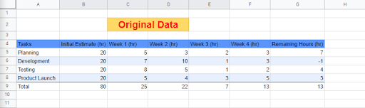
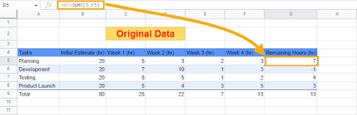
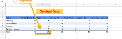
The “Remaining Hours” column represents the number of hours left to complete a specific task. Calculate this by taking away the sum of the total number of hours spent on a particular task category for each week from the estimated number of hours for that particular task category.
To get the values for the remaining hours in cell G5, use the formula =B5-SUM(C5:F5). Drag down to copy the formula to the cells below (G6:G8).
After creating the first table, proceed to creating the second table. The second table will have a Setting column and a column for each day/week/month within the product duration.
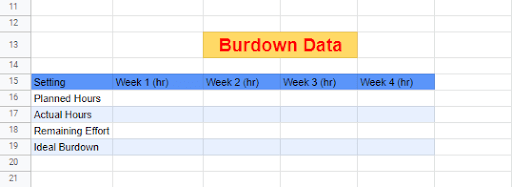
Entries in the second table are derived using calculated values from the first table. Let’s go over the details for getting each component’s values in the second table.
Planned Hours
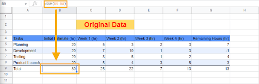
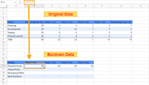
1. From the first table, take the sum of the values in the “Initial Estimate” column with the formula =SUM(B5:B8).
2. Reference the cell containing the summed value (B9) and divide by the number of weeks (4) using the formula =$B$9/4. Use the dollar ($) symbol to lock cell B9 before dragging the formula across to the other cells in the row (C16:E16).
Actual Hours
1. From the first table, take the sum of the total number of hours worked in the first week with the formula =SUM(C5:C8). Drag this across to get the total number of hours worked for each week (D9:F9).
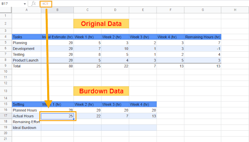
 2. In the second table, for the “Actual Hours” of Week 1, reference the cell containing the total number of weekly hours for the first week as calculated in the first table (C9). Drag this across to the other cells in the row (C17:E17).
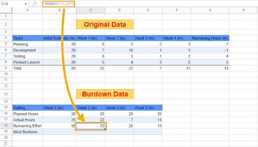
Remaining Effort
1. Subtract the total “Initial Estimate” ($B$9) from the total number of hours worked in the first week (B17). Use the formula =MINUS($B$9, B17).
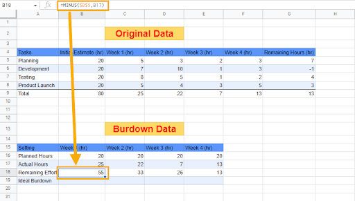
2. Subtract the number of hours worked in Week 2 (C17) from the value derived in the previous step (B18). Use the formula =MINUS(B18, C17). Copy this formula to the other cells in the row (D18:E18).
Ideal Burndown
1. Subtract the total of the “Initial Estimate” ($B$9) from the “Planned Hours” for the first week (B16) using the formula =MINUS($B$9, B16).
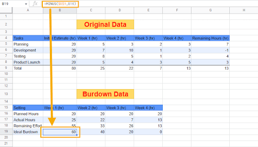
2. Subtract the “Planned Hours” value for Week 2 (C16) from the value derived in Week 1 (B19) using the formula =MINUS(B19, C16). Copy the formula to the other cells in the row (D19:E19).

Step 2: Insert a Combo Chart
After inspecting the data and creating the tables, the next step is to insert a combo chart. A combo chart uses a combination of bars and lines to visualize data.
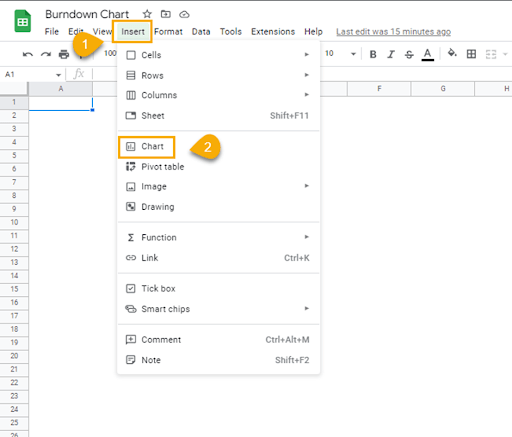
To add a chart, follow these steps:
1. Go to the Insert menu and click on Chart.
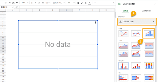
2. In the Chart editor window on the right side of the spreadsheet, under the Setup menu, go to Chart type. Click on the Column chart dropdown and select Combo Chart.
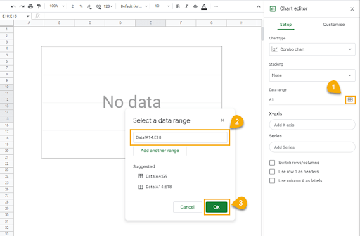
3. From the Chart editor window, go to Data range and click on the table icon. When the “Select a data range” dialogue box opens, go to the sheet containing the two tables and select the data in the second table.
Click OK.
At this point, you should have a chart that looks like this in your spreadsheet:
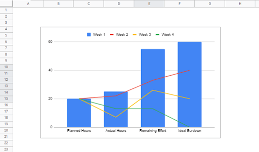
The chart needs a bit more modification because there are still a couple of things wrong with it. First, the chart plots the week’s numbers against the chart components when it should be the other way around.
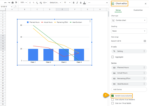
To use the week numbers as the X-axis, click “Switch rows/columns” in the Chart editor panel. This will cause the graph to plot the chart components against the week numbers.
Now, we want to get the Actual Hours to display in bars instead of lines. To do this, follow these steps:
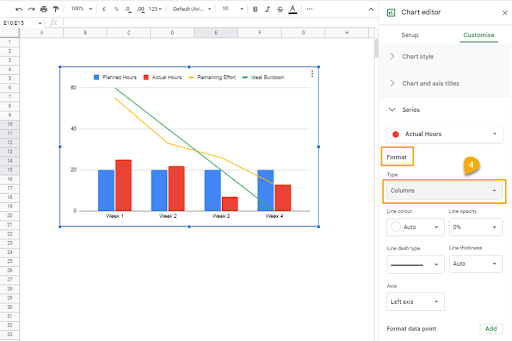
1. Click on the Customize tab.
2. Select Series.
3. From the dropdown, click “Apply to all series” and select Actual Hours.
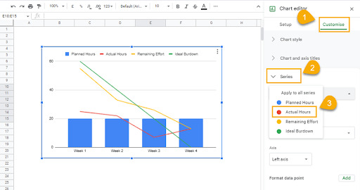
4. In the “Format” section of the Series dropdown options, click on the “Type” option and select Columns.
Now the bars display the Planned Hours and Actual Hours spent each week side-by-side, while the line shows the progress of the project in terms of the Remaining Effort and Ideal Burndown components.
How Do I Read a Google Sheets Burndown Chart
Earlier, we said a burndown chart uses four components to determine the progress of a project. To know how to read a burndown chart in Google Sheets, you must understand these components.
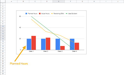
1. Planned Hours
This refers to the estimated number of daily/weekly/monthly hours necessary to meet a specific target. It is derived by dividing the total number of hours needed to complete the project tasks by the number of days/weeks/months to meet a specific deadline.
In the chart, the blue bars represent the planned hours.
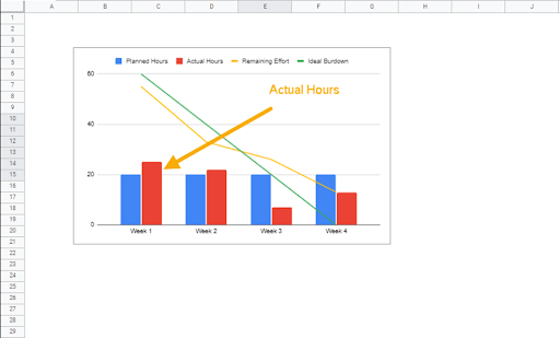
2. Actual Hours
This is the real number of hours spent per day/week/month working on project activities. In our example, the red bars in the chart represent the actual hours spent every week.
Plotted side-by-side with the planned hours component, you can see the times when the project team worked beyond expectations and when they fell behind.
With this, a project manager can use this information to identify what caused the drop in performance during these periods.
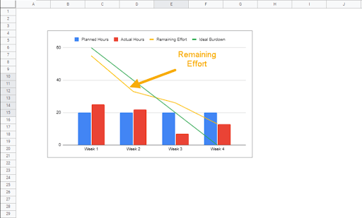
3. Remaining Effort
The remaining effort is the number of hours left to finish the project after the completion of a task for the day/week/month.
To get the value for the remaining effort, subtract the number of hours spent at the end of the day/week/month from the number of hours left to complete the project.
In our example, the project needs 80 hours, of which 25 hours were spent at the end of Week 1. The remaining effort after Week 1 is therefore 55 hours (80 – 25). Take away the number of hours spent in Week 2 (22) from 55, and this leaves 33. Continue this process until there are 13 hours still left at the end of Week 4.
The remaining effort provides insight into the work efficiency of a project team.
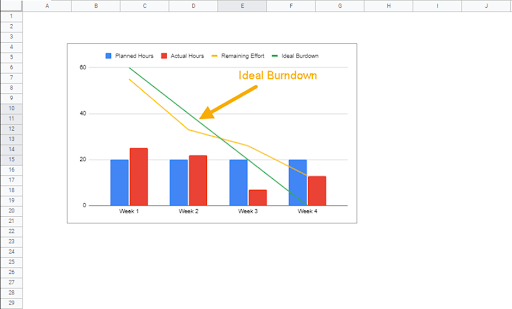
In the chart, the yellow line represents the remaining effort.
4. Ideal Burndown
The ideal burndown represents the number of hours expected to be spent on the project per day/week/month to meet the deadline if the situation was perfect.
It is derived by subtracting planned hours for each day/week/month from the remainder of the total estimated number of hours needed to complete the project within a given period. By the end of the last day/week/month, the ideal burndown value must be 0.
When plotted on a graph, the ideal burndown is usually a straight linear line and is generally plotted side-by-side with the remaining effort line for the sake of comparison. Together, these two measures are useful for making important decisions necessary for keeping a project on track.
From our example, the green line represents the ideal burndown.
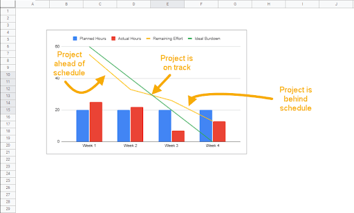
When the remaining effort line is below the ideal burndown line, it indicates that the project is ahead of schedule.
This is because, at the point where the remaining effort line is below the ideal burndown line, more hours have been spent working than was ideally stipulated.
When the remaining effort and the ideal burndown lines intercept, it indicates that the project is right on schedule. At that point, the cumulative number of hours spent working per day/week/month is equal to the cumulative number of hours expected to be spent in an ideal situation.
As soon as the remaining effort line starts to creep above the ideal burndown line, the project is already falling behind schedule. This means that the number of hours spent at that point is less than the number of hours that are expected to have been spent if the project is going to meet any stipulated deadline.
When Should I Use a Burndown Chart in Google Sheets?
There are various situations wherein you can find a use for a burndown chart in Google Sheets. Some of the burndown chart common uses cases are as follows:
1. You can use a burndown chart to determine the level of employee commitment to a project.
2. When your team frequently misses deadlines, the burndown chart can provide valuable insight into understanding the reason behind this.
3. The burndown chart can also help you to identify how much time a project requires and when it will be completed.
