
The If Greater Than and Less Than function in Microsoft Excel is a logical function that returns one value if the conditions are met and another value if the conditions are not met. This function is useful for making decisions based on data in your spreadsheet.
How to Use If Greater Than and Less Than in Excel
The Greater Than and Less Than symbols in Excel are used to compare two values. If you want to know if a number is greater than or less than another number, you can use the Greater Than (>) and Less Than (<) symbols.
You can also use the Greater Than or Equal To symbol, which is represented by the >= symbols. This will return TRUE if the number you are testing is greater than or equal to the number to which you are comparing it. For Less Than or Equal To, use the <= symbols.
You can also use the Not Equal To symbol, which is represented by the <> symbols. This will return TRUE if the number you are testing is not equal to the number to which you are comparing it.
Here are some examples of how these symbols can be used in Excel.
Using the OR Function
The OR function is a logical function in Excel that returns TRUE if any of the condition’s arguments are TRUE and FALSE if all the arguments are FALSE.
Let’s take a look at how to set up the OR Function with the Greater Than and Less Than symbols.
1. Click on the cell where you need your result.
2. Go to the Formula bar and type =OR(A2<5, B2<5). Here, A2 and B2 are the cells with our values, and 5 is the number for the condition to which you are comparing your values.
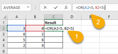
3. Press the Enter key on your keyboard.
4. Drag the cell down to apply the formula to the remaining cells.
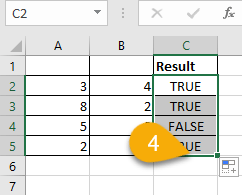
There you go!
Using the AND Function
The AND function is a logical function that returns TRUE if all of the conditions are satisfied and FALSE if any of the conditions are not met, even if some of them are.
To use this function, do the following:
1. Select the cell where you want your result.
2. In the Formula bar, enter =AND(A2<10, B2<10), where A2 and B2 are the cells with your values, and 10 is the condition to which you are comparing the numbers.
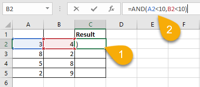
3. Hit the Enter key on your keyboard.
4. Drag the cell with the formula down through the rest of the cells to copy the formula into the other cells.
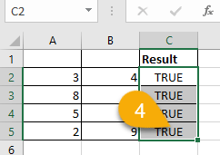
Voila! You’ve effectively employed the Less Than symbols in this example.
Using the IF Function with the Greater Than or Less Than Symbols
The IF function in Excel is a logical function that is used for making decisions. The function checks whether a certain condition is met, and if it is, then it returns a particular value; otherwise, it returns another value. The condition that you specify is compared to your values using the greater than (>), less than (<), or equal to (=) symbols.
Let’s dive in and see how you can use it! Here is one example of the IF function with the Greater Than or Less Than symbols:
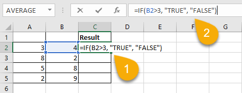
1. Click on the cell where you want your result.
2. Navigate to the Formula bar and enter =IF(B2>3, “TRUE”, “FALSE”). B2 is the cell with your value, and 3 is your condition to which you are comparing your value. If the condition is met, it will show TRUE. If the condition is not met, it will show FALSE.
3. Press Enter.
4. Copy this formula into the remaining cells by dragging the initial cell with the formula downward through the rest.
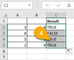
Here is the result!
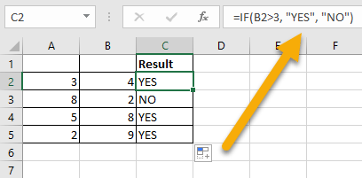
NOTE: You can replace the terms “TRUE” and “FALSE” to anything you want to match your needs (such as “YES” and “NO”). Just be sure to keep quotation marks in the formula around the words you want to use.
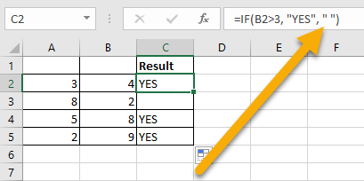
You can also omit one of the values in your formula if you want to leave the cell blank. See the below example:
Using the SUMIF Function
The SUMIF function in Excel is used to sum up the cells that meet certain criteria. For example, you can use the SUMIF function to sum up all the cells in a range that are greater than or less than a certain value.
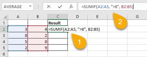
1. Select the cell where you want your result.
2. In the Formula bar, type =SUMIF(A2:A5, “>8”, B2:B5). Here, A2:A5 and B2:B5 represent the range of your cells. 8 is the conditional number to which you will compare the values.
3. Hit the Enter key on your keyboard.
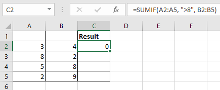
Here you can see that the requirement has not been satisfied, which is why the result is zero.
Using the COUNTIF Function
The COUNTIF function in Excel is a logical function that determines how many cells fulfill the criteria you provide.
Let’s see how to apply it.
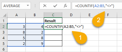
1. Pick the cell where you want your result.
2. Navigate to the Formula bar and type =COUNTIF(A2:B5,”<>”), where A2:B5 is the range of cells to which you will apply the formula.
3. Press the Enter key.
4. Drag the cell downward to apply the formula to the remaining cells.
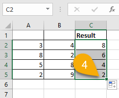
Easy peasy!
The Greater Than and Less Than symbols in Excel are used to compare values and return a result. You can use these symbols to calculate if a value is greater than or less than another value or to compare two ranges of values.
