
The IF function is one of the most popular and widely used functions in Excel. It allows you to test a condition and return one value if the condition is TRUE and another value if the condition is FALSE. Using the IF functions with multiple conditions allows you to craft sophisticated formulas to perform complex tasks.
In this article, we’ll take a look at a variety of functions that work well with the IF function!
IF Function
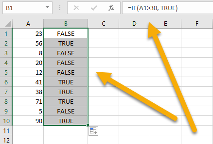
Firstly, let’s look at the IF function with one condition. In this situation, we will use the =IF(A1>30, TRUE) formula, where A1 is the cell with the starting value. After applying the condition to A1, you can drag the cell with the formula downward to copy the formula and see the result in the other cells. We can see below how the function worked.
IF with Multiple AND Operations
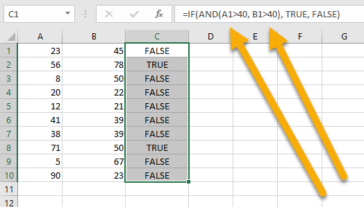
The AND operator is a logical function that may be used to evaluate multiple conditions at the same time, meaning every condition must be met to return a TRUE result. If you have, for example, two columns of metrics, you can use the =IF(AND(A1>40, B1>40), TRUE, FALSE) formula. In this example, the condition is applied to two separate cells, and the conclusion is derived from the two values. Here, A1 and B1 are the cells with the values being evaluated.
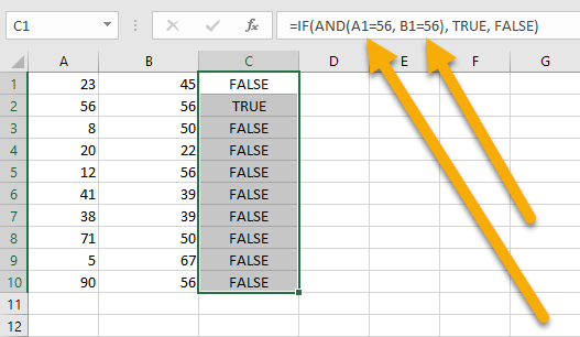
Another formula you can apply is =IF(AND(A1=56, B1=56), TRUE, FALSE). The value of our condition is 56, which corresponds to both cells (A1 and B1). To get a TRUE result, both cells will have to equal 56. You can use text and symbols. It makes no difference in this case.
Let’s move on and consider other IF functions with multiple conditions!
IF with Multiple OR Operations
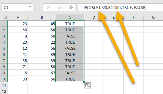
The OR function is a logical function in Excel that determines whether any of the conditions being examined are satisfied. In other words, it examines to see if at least one condition is true, even if the others are not.
Below, we use the =IF(OR(A1>20, B1<50),TRUE, FALSE) function, where A1 and B1 contain the values to be evaluated.
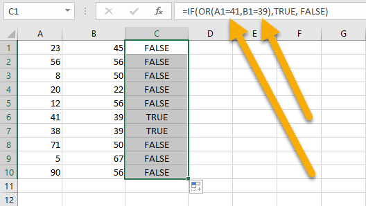
Here is another formula with other conditions: =IF(OR(A1=41,B1=39),TRUE, FALSE). Let’s see the result!
IF and the CONCATENATE Function
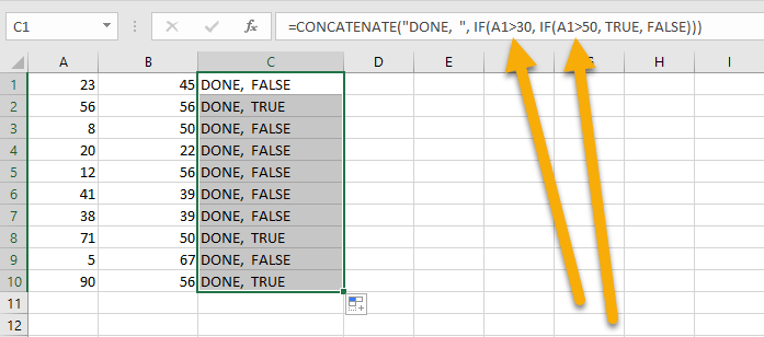
The CONCATENATE function, which is a built-in function in Excel, takes two or more pieces of text and combines them into one cell. In our case, the formula =CONCATENATE(“DONE, “, IF(A1>30, IF(A1>50, TRUE, FALSE))) shows how the CONCATENATE function works. A1 is the cell with the value being tested by the formula. DONE, TRUE, and FALSE are the indicators of the obtained result.
IF with the ISNUMBER, ISTEXT, and ISBLANK Functions
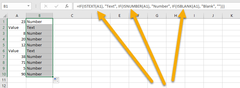
The ISNUMBER, ISTEXT, and ISBLANK functions demonstrate whether the cell contains a number, text, or nothing. As a consequence, the results are determined by what’s in the specified cell. Here, we use the following formula: =IF(ISTEXT(A1), “Text”, IF(ISNUMBER(A1), “Number”, IF(ISBLANK(A1), “Blank”,””))). Here’s an example to illustrate that:
IF with SUM and AVERAGE Functions
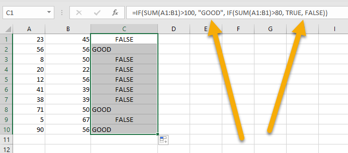
The SUM function in Excel is a built-in function that adds up the values in a range of cells, although you could set it up to add only those cells that fulfill specific criteria. In the case below, we have used the formula =IF(SUM(A1:B1)>100, “GOOD”, IF(SUM(A1:B1)>80, TRUE, FALSE)), where A1 and B1 are cells with your values. GOOD, TRUE, and FALSE are the conditions. Here we’ve got the result:
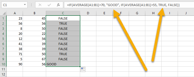
Alternatively, you can use the AVERAGE function. The formula we used below is =IF(AVERAGE(A1:B1)>70, “GOOD”, IF(AVERAGE(A1:B1)>55, TRUE, FALSE)). A1 and B1 contain your values. There are three conditions here: GOOD, TRUE, and FALSE.
IF with MIN and MAX Functions
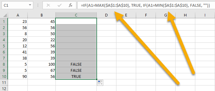
The MIN and MAX functions are used to find the minimum and maximum values in a data set. These functions are often used together to create dynamic ranges. Use the formula =IF(A1=MAX($A$1:$A$10), TRUE, IF(A1=MIN($A$1:$A$10), FALSE, “”)), where A1:A10 is your cell range and TRUE and FALSE are the conditions. Here is the result:
IF Function FAQs
Let’s go through a few questions to help you learn more about the IF function.
How does the IF Function work in Excel?
The IF function in Excel can be used to test for multiple conditions. When using the IF function, you need to specify three arguments: the logical test that you want to perform, the value that you want to return if the logical test is TRUE, and the value that you want to return if the logical test is FALSE.
What is the IF Function used for?
The IF function is one of the most popular functions in Excel. You can use the IF function with multiple conditions by nesting the formula. This is known as nesting because you’re putting one IF function inside another.
For example, you might want to test multiple conditions and return a different result for each condition. In this case, you would nest an IF function inside another IF function.
