
If you are a working professional, you are likely looking for better budget planning to make sure you are not overspending on things that are not important, especially in the context of your salary.
Though many tools in the market allow you to track your budget and expenses, most either charge money (again, unnecessary spending) or lack a few components you wish they had.
You might be surprised to learn that you can easily create a budget tracker template for Google Sheets.
Yes, this is absolutely possible, and this article will show you how!
Follow the steps below to see how easy it is to create this tool—and the beautiful thing is that you don’t need to spend money on those expensive budget tools in the market.
Template Overview
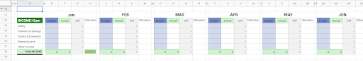
Take a look at this Budget and Expense Calculator template you can create in Google Sheets:
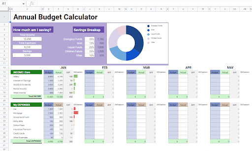
With this tool, create Income and Expense categories and add rows to each to customize the list according to your personal lifestyle.
Review the difference between your Budget and Expenses through the Diff column, while the Utilization column provides a small pictorial infographic with the help of a custom formula to show how your Income and Expenses move across each category. This also gives you a glimpse of important sources of income and key expense categories that you should keep an eye on.
Finally, at the top of the sheet, create your own analysis of your Income and Expenses: how much you are saving, where to put your savings based on certain categories, and a visual representation of your savings.
Creating the Income and Expense Categories
Now let’s see how to make our own from scratch. Open a new blank spreadsheet where you wish to create the Budget and Expense Calculator.
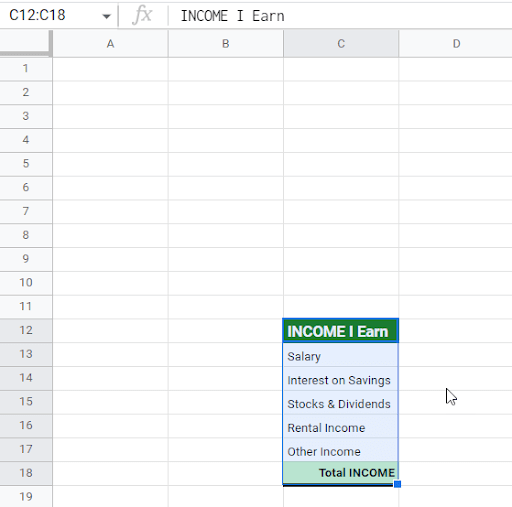
Step 1. In cell C12, Type “INCOME I Earn” as the column header. This section will contain your income categories. Below the header, type the income categories that apply to your situation. You can see our examples in the screenshot below.
Formatting:
a. The font style for this particular template is Roboto, with the header set at font size 10 and all other cells at font size 8. This will be the standard format throughout this sheet.
b. For cell C12, the font color is white, and the cell color is Close to dark green 2 from the color options (hexadecimal code #1d7e1d).
c. Set the cell color for Total INCOME to Close to light green 13 (hex code #cdf3cd).
d. Add a thick Bottom Border for the Total INCOME cell.
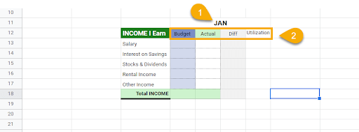
Step 2. In the columns to the right of column C, create 12 categories for months across the year. The headers should read JAN, FEB, MAR, …, and DEC, with all the headings listed across row 11.
Step 3. Below each month, set up four columns representing Budget, Actual, Diff, and Utilization, respectively.
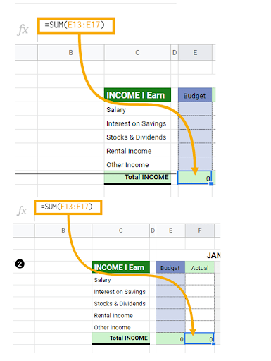
Step 4. In cell E18, type in the formula =SUM(E13:E17), which allows you to generate the total for the Budget column. Repeat this process to create the total for the Actual column using the formula =SUM(F13:F17).
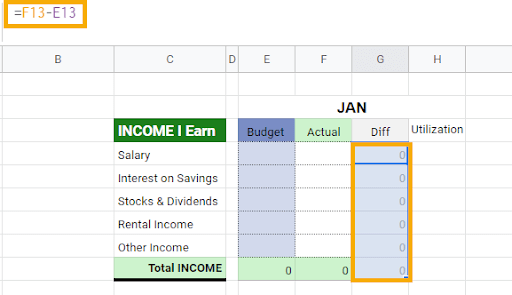
Step 5. The Diff column represents the difference between the Actual and the Budget columns. Type the formula =F13–E13 in cell G13 to calculate this difference and drag the formula down the column to G18.
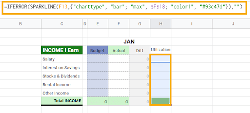
Step 6. For the Utilization column, we will create a Data-Bar-like structure to show the actual income compared to the budget amount. To create this, copy and paste the following formula in cell H13 and drag it down the column to H18.
=IFERROR(SPARKLINE(F13,{“charttype”, “bar”; “max”, $F$18; “color1”, “#93c47d”}),“”)
The SPARKLINE function allows you to add pictorial graphs in the cells. Set the initial data value to cell F13, which represents the Actual income from the Income Category Salary. Note that there is a blank column (D) between Income I Earn and Budget to improve readability.
For the SPARKLINE options, create an array in which charttype is set to bar chart, the max value is set to the Total value of column Actual ($F$18), and the color is set to Light green 1, with hex code #93c47d.
Formatting:
a. Resize the monthly Budget, Actual, Diff, and Utilization columns to a column width of 50. Set the width of column D to 10 units.
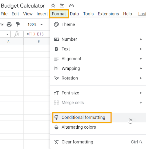
b. For the Diff column, apply conditional formatting to each row, changing the text color from gray to black when the difference value is greater than 0.
c. Navigate to the Conditional formatting option through the Format menu from the uppermost ribbon.
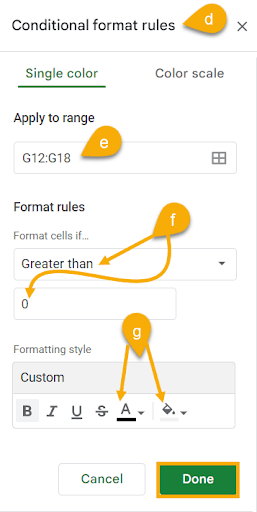
d. When the Conditional format rules window pops up, click Apply to range and set the range as G12:G18. This applies the conditional formatting to that range.
e. Under the Format rules section, select Greater than through the dropdown. In the text box that appears below this dropdown, type in 0.
f. Finally, under Formatting style, set the Text color to black and the Fill color to Close to light gray 3 (#f2f2f2). Don’t forget to click on the Done button to apply these changes.
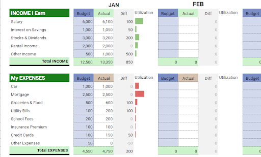
Step 7. Copy this entire setup for each month of the year. This layout now shows a monthly income breakdown for the entire year. The final layout should look like this:
Step 8. Using the same formatting, create the My EXPENSES section. List your expenses and repeat the Budget, Actual, Diff, and Utilization columns for each year. The only difference is that the Utilization formula has the bar color set to Light red 1 (hex code #e06666). See the screenshot below:
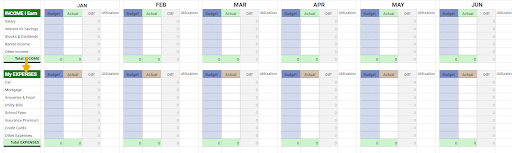
Note: The Car, Mortgage, Groceries & Food, etc., are some common expense categories, but feel free to modify them to fit your own list of expenses. You can add rows above the final Total EXPENSES row for additional categories.
Adding Additional Layout to the Report
Now that you have the basic layout ready for your Budget and Expense Tracker tool, let’s add a few more details to personalize your report.
We’ll look at adding a title to the report, a few essential budget and expense highlights that pop up as soon as you open this tool, and an excellent infographic that will visualize where your savings are going. The area we will use for this falls in the first ten rows that we kept blank intentionally.
Step 1. Type the title for your report (such as Annual Budget Calculator) in the first row of column C (cell C1). It will describe this tool and serve as a header for this calculator.
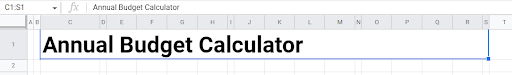
Here is the formatting we used here:
Font size = 30 (so the header really stands out) and make it bold.
Merge cells C1:S1 to populate this header across those rows.
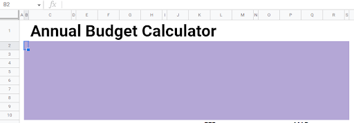
Step 2. Starting from cell B2 to S10, make a selection and set the Fill (or Cells) color to Light purple 2. This is where you will add a few key performance indicators (KPIs) related to this calculator.
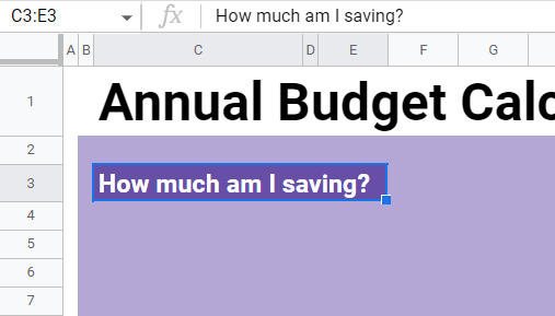
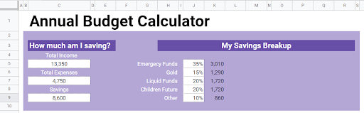
Step 3. In cell C3, type the header How much am I saving? This section is specifically designed to demonstrate how much you are saving from your total annual income. Merge the title across C1 to E1. Make it bold, and the Font should be Roboto at size 14.
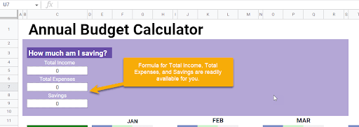
Step 4. Now add three new categories, one below another, for Total Income, Total Expenses, and Savings. Each of these fields will produce a value based on the following formulas:
Total Income =SUM($F$18,$K$18,$P$18,$U$18,$Z$18,$AE$18,$AJ$18,$AO$18,$AT$18,$AY$18,$BD$18,$BI$18)
Total Expenses =SUM($F$29,$K$29,$P$29,$U$29,$Z$29,$AE$29,$AJ$29,$AO$29,$AT$29,$AY$29,$BD$29,$BI$29)
Savings
=C5–C7
If you dig the formula for Total Income down, you will find that it is the sum of the Actual column for Income for each month. The same goes for Total Expenses, which is the sum of the Actual column for Expenses for each month. Finally, Savings is simply the difference between Income and Expenses.
Step 5. Across cells H3 to R3, add the header My Savings Breakup, merging cells as needed, as shown in the screenshot below. The data itself will span across cells H5:K9.
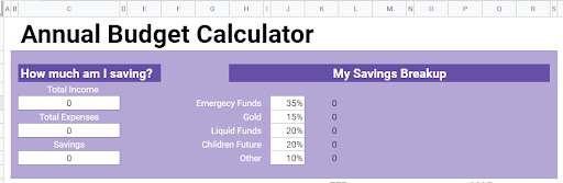
The idea is to allocate your savings into different categories. As a wise man once said, don’t put all your eggs in one basket. Column K will use a formula that breaks down the Savings amount based on percentages for each category:
=J5*$C$9
Right now, the result is zero because there aren’t any values for monthly income and expenses yet in the table below.
Step 6. To make this layout work, let’s add some values for JAN, both Budget and Actual for the Income and Expenses categories. The values input below are imaginary, but be sure to add your actual data to your copy. The formulas will never break (until you mess with them!).
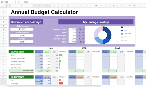
Step 7. Now, take a look at the KPI section above this table. It will make more sense as you can see the Total Income, Total Expenses, and Savings along with your savings breakup across the different categories based on the percentages you assigned to each category.
Step 8. Use this savings breakup to create a nice-looking pie chart that visually displays how you allocate your savings to the different categories.
The final layout should look like the one shown below:
Notes:
1. You can set the Income and Expense values for both the Budget and Actual columns. Experiment with this tool to see how it works with different value combinations.
2. You can also change the percentage breakdown for different savings categories. For example, someone may choose to put 20% into Emergency Funds and add more weightage to Gold. This is absolutely fine; the tool is flexible enough to allow you to change those percentages.
3. Never change the formulas under any circumstances; otherwise, this tool may not work as expected.
Creating Budgets in Google Sheets: FAQs
Let’s look at some frequently asked questions for this topic.
Does Google Sheets have a budgeting tool?
Put simply, NO!
Google Sheets doesn’t have a budgeting tool of its own. However, many versions of budgeting tools developed by people like us are freely available as templates. You can find those on the Google Marketplace ready to download and use or search for them on Google.
How do I make a budget in Google Sheets?
If you are interested in creating a budget tool of your own but don’t know where and how to start, read through the step-by-step article above. If you follow the steps here, you can create your very own visually appealing Budget and Expense Tracker.
Does Google Sheets have a budget template?
Google Sheets does not have a prebuilt budget template. However, you can search thousands of budget templates on Google Marketplace, ready-made and available for budget and expense tracking from the word go!
