
To use the TRANSPOSE function in Google Sheets, select your data, right-click on it, and choose the Copy option. Next, right-click on a blank cell, select Paste special, and pick the Transposed option.
This guide covers everything you need to know about the Google Sheets TRANSPOSE Function: its definition, syntax, use cases, examples, and usage notes.
How to Quickly Transpose Data in Google Sheets
The TRANSPOSE function in Google Sheets allows you to move data between ranges of cells. Let’s take a look at how this can be done with just a few steps.
Difficulty: Beginner
Time Estimate: 7 seconds
- Select a blank cell.
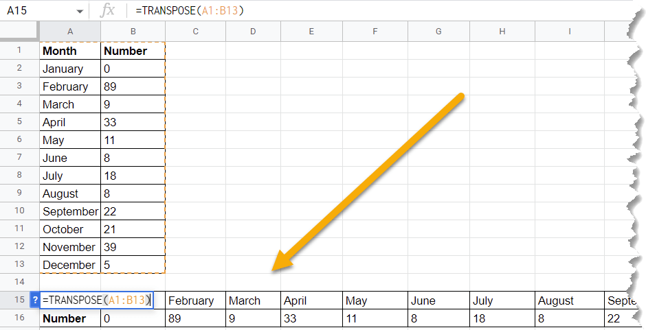
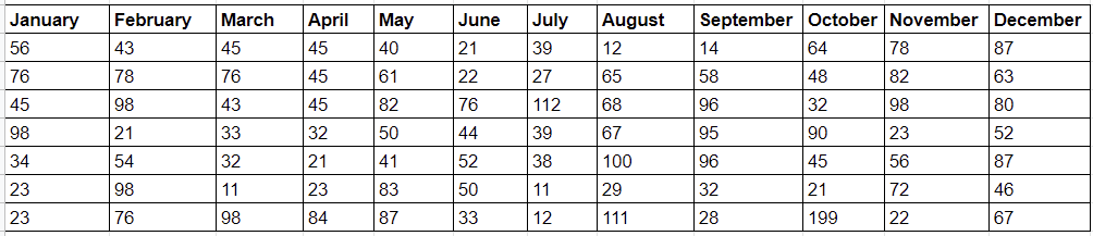
- Go to the Formula bar and type the formula =TRANSPOSE(A1:B13). A1:B13 is the cell range you need to move.
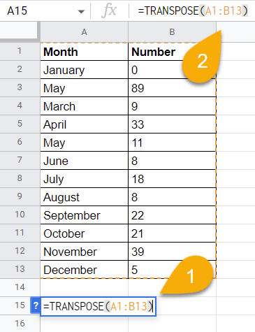
- Hit the Enter key.

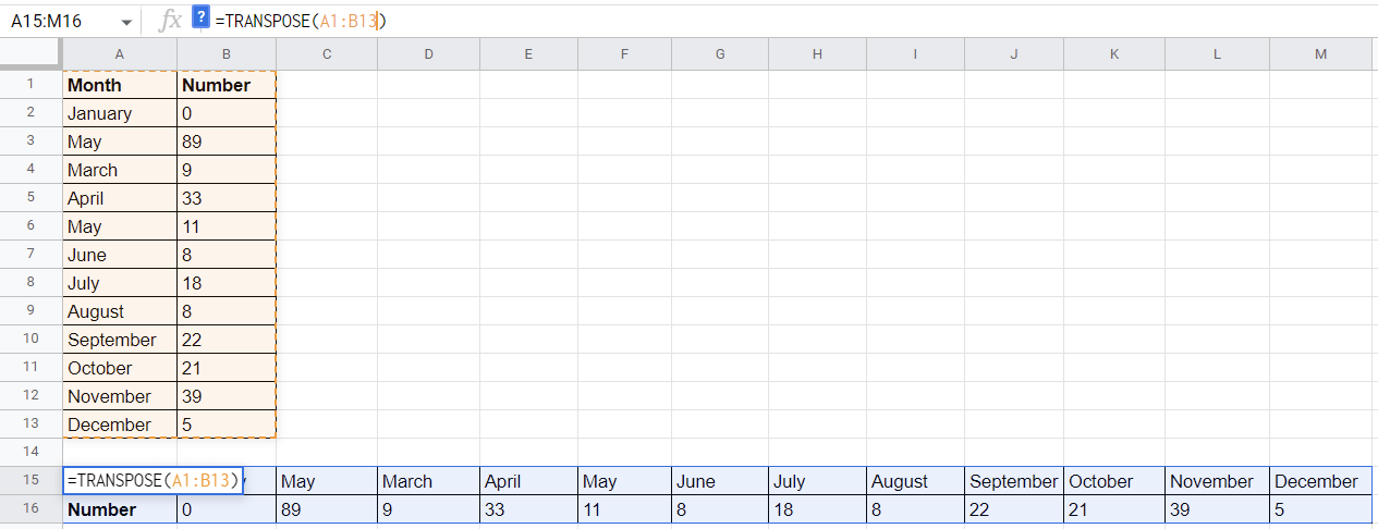
Here is the result!
Drilling Down into the TRANSPOSE Function
Description
The TRANSPOSE function is a Google Sheets function that allows you to transpose data from one range of cells to another.
For example, if you have data in a column, you can use the TRANSPOSE function to move it to a row. Or, if you have data in a row, you can use this function to move it to a column. The TRANSPOSE function allows you to rotate data from a horizontal orientation to a vertical orientation or vice versa.
The following example of the function =TRANSPOSE(A1:B13) shows how it works.
Purpose
This function helps you reposition your data to make it easier for you to navigate through the information. It is used to rearrange data in a certain order or if you want to change the structure of your data.
Syntax
=TRANSPOSE(array_or_range)
Arguments
- array_or_range is the specified array or range to be moved.
Return Value
Using the TRANSPOSE function, a vertical range of cells can be returned as a horizontal range or vice versa.
Usage Notes
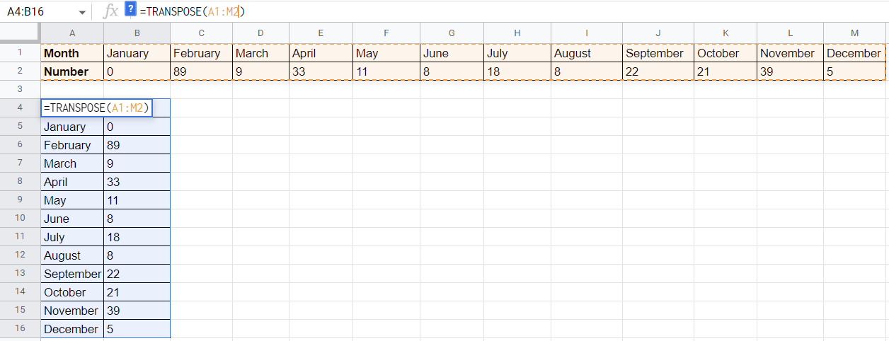
- Using this function, you can display your data horizontally.
- Conversely, the application of this function can arrange data in a vertical position.
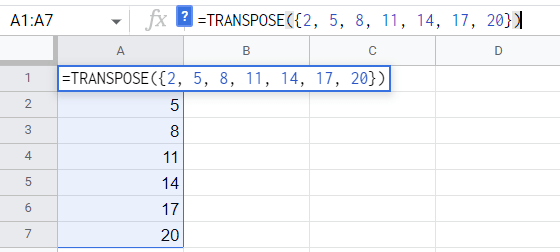
- If you don’t intend to select a range of cells with data but just want to enter a function with your values, you need to add curly brackets to the formula, as shown in the example below.
Examples
Here are some examples we have used. It is necessary to enter your own range in the formula for the function to work.
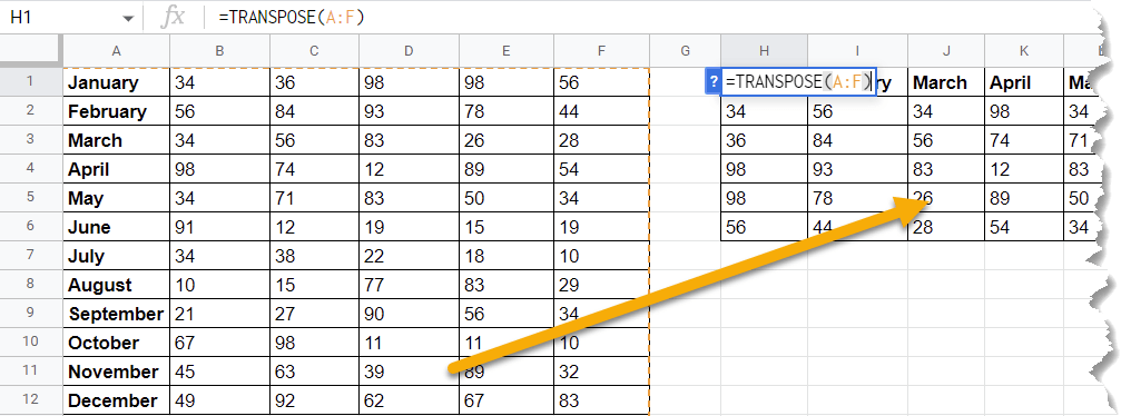
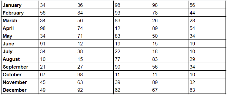
- If you need to transpose columns, use the formula:
=TRANSPOSE(A:F) // Output:
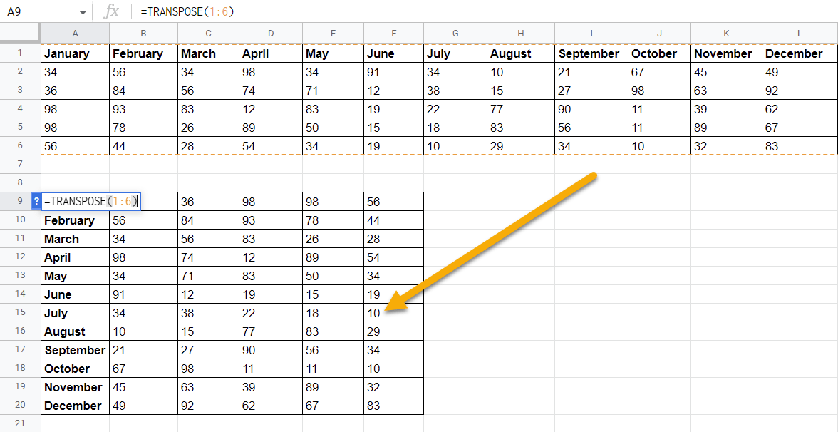
- The following example demonstrates how to transpose rows:
=TRANSPOSE(1:6) // Output:
- If you need to transpose cell ranges, use the following:
=TRANSPOSE(A1:B13) // Output:
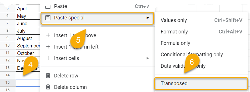
Bonus: Transpose Data Using the Paste Special Option
Difficulty: Beginner
Time Estimate: 5 seconds
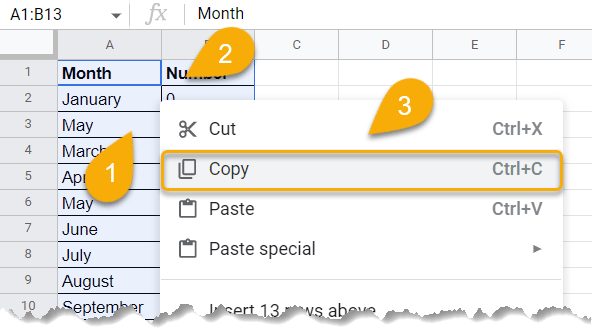
- Highlight your data.
- Right-click on it.
- Choose the Copy option.
- Next, right-click on a blank cell.
- Pick Paste special.
- Finally, select Transposed.
Voila! You have done it!
The TRANSPOSE Function in Google Sheets FAQs
If you are interested in finding out more, take a look at our FAQ section!
Can you transpose multiple columns in Google Sheets?
Yes, you can transpose multiple columns in Google Sheets. To do so, you’ll need to select a blank cell, and in the Formula bar, type =TRANSPOSE(A:L). A:L is the columns’ range. Then press Enter.
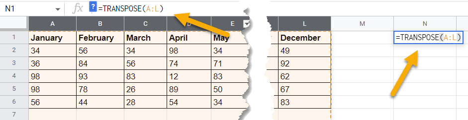
And that’s it! The values from the selected columns will now be transposed into the new rows.
How do I transpose multiple rows to columns in Google Sheets?
To transpose multiple rows to columns in Google Sheets, click on the cell where you want the result, go to the Formula bar, type the formula =TRANSPOSE(1:12), where 1:12 is the row selection, and hit Enter.
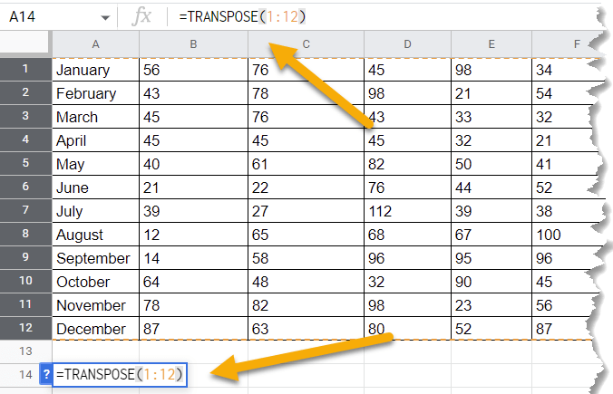
It’s as simple as that.
Is there a shortcut to quickly apply the TRANSPOSE function?
Yes, there is a keyboard shortcut that you can use to apply the TRANSPOSE function in Google Sheets. To do this, select your data and press Ctrl + Shift + V on your keyboard.
Keep in mind that using this shortcut will permanently change your data, so be sure only to use it when you’re absolutely sure you want to transpose your data.
Why is TRANSPOSE not working in Google Sheets?
In the case that the TRANSPOSE function isn’t working, there are several factors that could be causing this to happen:
- One of the reasons why this happens is because the cell that you selected already contains data in it. In this case, you will see the following warning.
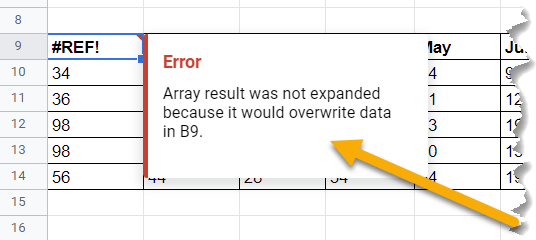
To solve this problem, make sure the cells where you intend to transpose the data are empty.
- Also, if you have merged cells, this function may not work or may not transfer the corresponding cell with data.
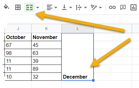
Make sure the cells are not merged before applying the formula.
