
Excel Half Pie Chart Template – Free Download
A half pie chart (also known as a semicircle or half-moon chart) is a 180-degree version of a basic pie graph that illustrates the relative sizes of data. This brief guide will teach you how to quickly create this half pie chart in Excel:
Sample Data
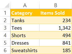
Consider this simple table containing the sales of a fictitious clothing store sorted by category:
Now, let’s get down to business.
Step 1. Add a Dummy Data Series
The whole trick here is to create a dummy data series that will take up half of a full pie chart and make that slice invisible to get exactly what we’re looking for.
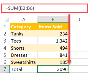
To do that, start with setting up a dummy data series that contains the sum of all of the actual values in your data table by using the SUM formula.
- Type “Total” into A7.
- Enter “=SUM(B2:B6)” into B2.
Step 2. Create a Simple Pie Chart
The chart data is ready to go, meaning it’s time to build a regular pie chart.
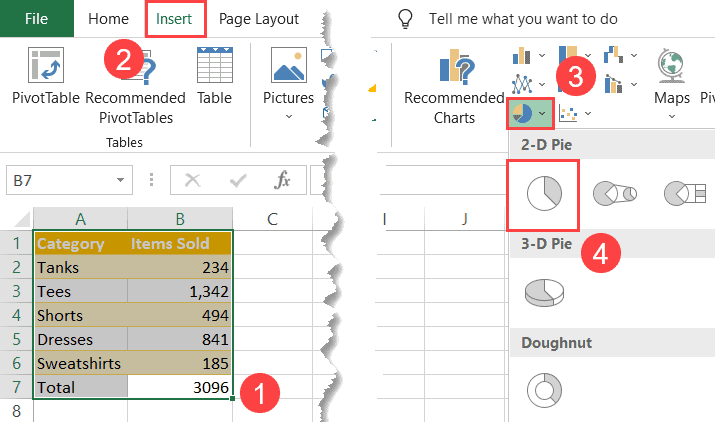
- Highlight the expanded data table (A1:B7).
- Go to the Insert tab.
- Click “Insert Pie or Doughnut Chart.”
- Hit the “Pie” button.
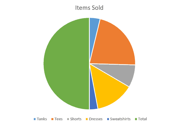
Here’s what you should end up with by the end of this step.
Step 3. Hide the Dummy Series
Your next step is to make the dummy series invisible, effectively getting a half pie chart.
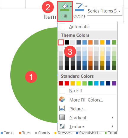
- Double-click on Series “Total” represented by the largest slice of the pie chart.
- Click the “Fill” button.
- Pick white from the color palette.
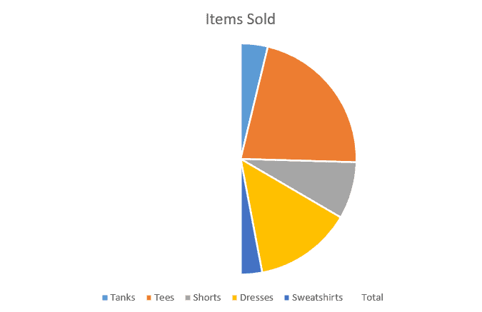
Here’s the result:
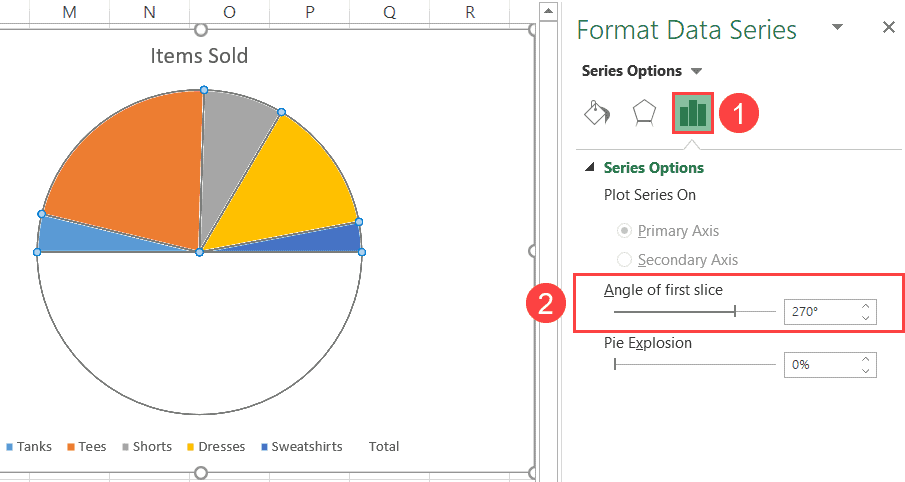
Step 4. Rotate the Half Pie Chart
Technically, you’re good to go, but if you want to rotate the half-moon chart to make it a bit more accessible, here’s how you do that.
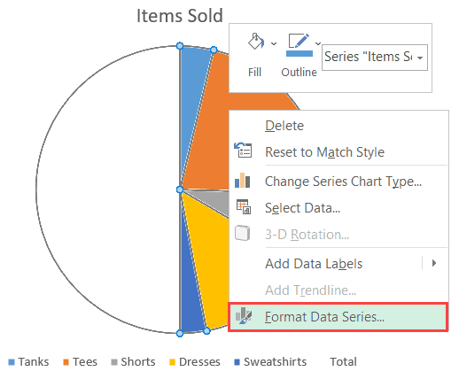
Right-click on your half pie chart and select “Format Data Series” from the menu that pops up.
- Switch to the Series Options tab.
- Change “Angle of first slice” to “270°” or “90°.”
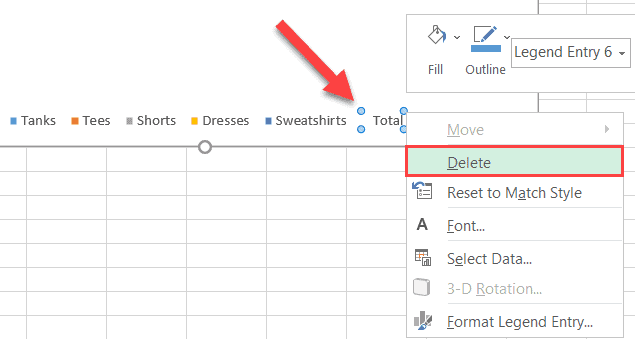
Step 5. Clean up the Chart Legend
Finally, remove the legend label related to the hidden slice of the pie chart. To do that, right-click on the label that reads “Total” and click “Delete” to erase it.
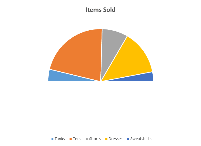
Check out the final result – once you have finished the last step, your semicircle chart is ready to go.
