
A pie chart (also known as a circle chart) is a circular graph where each slice illustrates the relative size of each element in a data set.
Stick around to learn all about how to quickly build and customize pie charts.
Also, we have a separate guide covering how to make a pie chart in Google Sheets.
How to Make a Pie Chart in Excel in Less Than 60 Seconds
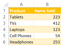
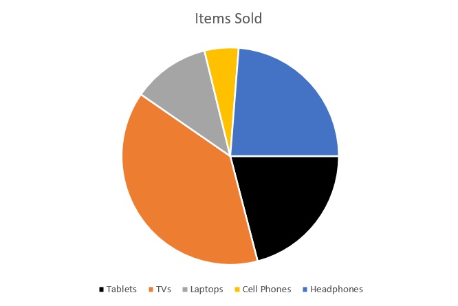
Without beating around the bush, let me show you the easiest and fastest way to build circle charts. Here’s some dummy data we’re going to use:
Read More: How to Create an In-cell Pie Chart in Excel
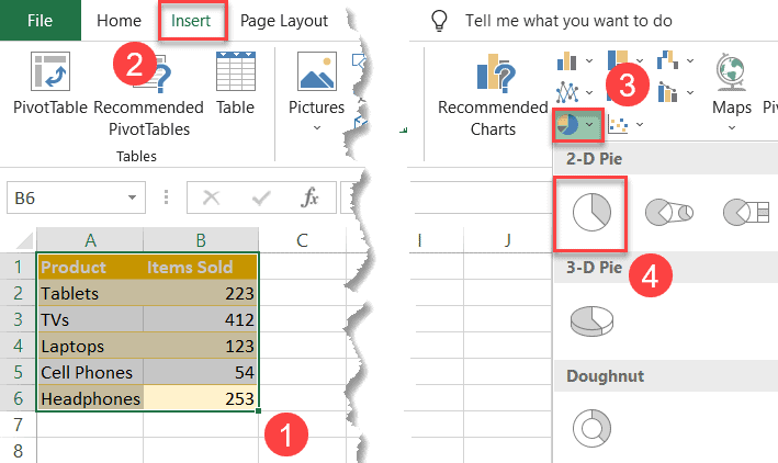
To build a pie chart with that data, all you need to do is follow a few simple steps:
- Highlight the entire data table (A1:B6).
- Go to the Insert tab.
- Click “Insert Pie or Doughnut Chart.”
- Choose “Pie.”
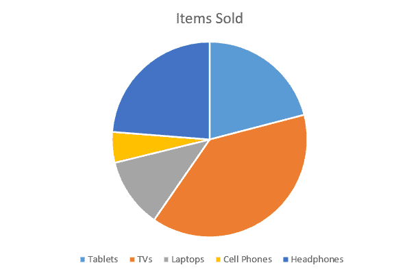
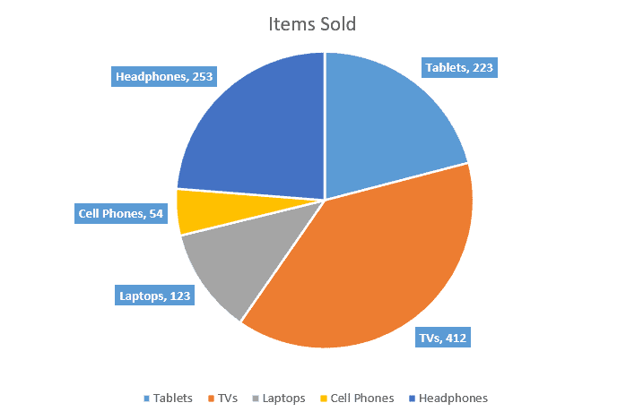
Ta-da! There you have your pie chart.
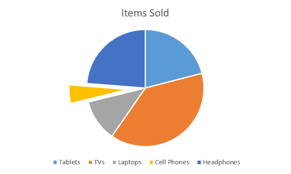
But here’s more to it than that. If you want to explode a single slice of your pie chart, just double-click on the slice you want to explode and drag it away from the chart center.
Using a similar process, you can create a male/female pie chart in Excel.
Related Article: How to Create a Panel Chart in Excel
How to Add Labels to a Pie Chart
To make our circle chart a bit more informative, add some data labels illustrating the numeric value of each slice by right-clicking on your pie chart and choosing “Add Data Labels.”
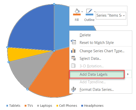
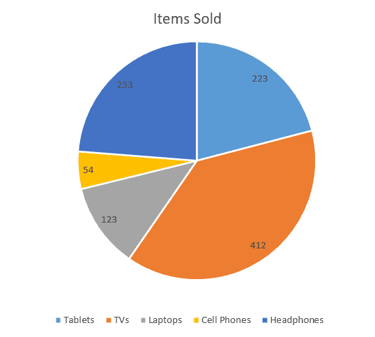
Once there, Excel will automatically generate dynamic data labels based on your actual values.
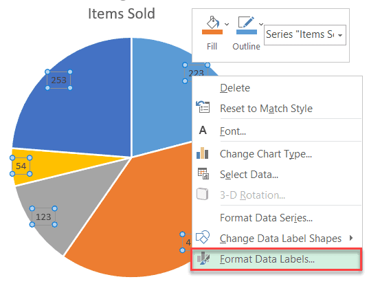
The default data labels just don’t cut it, so let’s customize them a bit to make the chart more visually appealing.
To start with, right-click on any of the data labels and choose “Format Data Labels.”
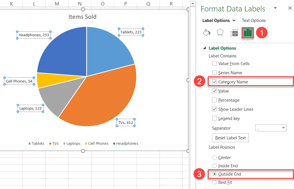
In the task pane that appears, do the following to spruce up your data labels:
- Navigate to the “Label Options” tab.
- Under “Label Options,” select “Category Name” to display the product categories next to the actual values.
- Under “Label Position,” click “Outside End” to push the labels outside the pie chart.
Having changed the font and background color of the labels on top of those tweaks to other chart elements, here’s how our pie chart should look like now. Additionally, consider rotating your Excel pie chart to make your data stand out.
The “Label Options” tab provides a whole host of customization options to create professionally-looking pie charts using basic Excel features and tools.
Read More: How to Create a Half Pie Chart in Excel
How to Change Pie Chart Colors
To quickly change the color of the slices in your pie chart, here’s what you need to do:
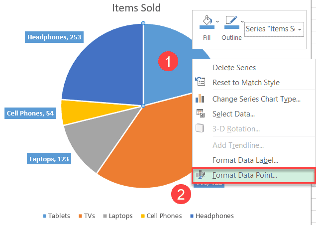
- Double-click on the slice you want to modify.
- Click “Format Data Point.”
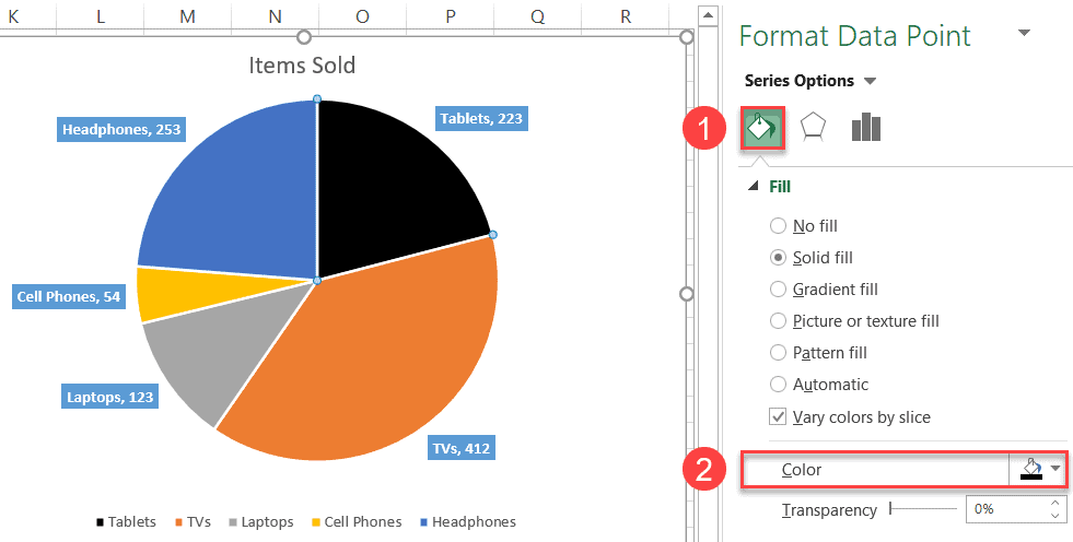
- Go to the “Fill & Line” tab.
- Click “Fill Color” and choose black from the color palette.
‘
Now, over to you! You now have all the information you need to build stunningly beautiful circle graphs in Excel.
How to Rotate a Pie Chart
In order to rotate a pie chart without messing up the chart title and legend, do the following:
1. Right-click on your pie chart and pick “Format Data Series” from the menu that appears.
![]()
2. Go to the “Series Option” tab.
3. Set the “Angle of first slice” value to “90°” to rotate the chart 90 degrees clockwise – and the great news is that you can tweak the value however you want.
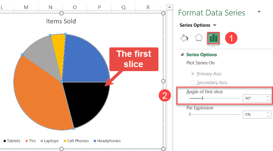
Having followed the simple instructions outlined above, you rotated the X and Y-axis by 90 degrees without affecting the rest of the plot.
Pie Chart in Excel – Free Template
Short on time? Grab our free Excel pie chart template to get up and running in less than a few clicks.
Excel Pie Chart Template – Free Download
FAQs
What is an Excel Pie Chart?
An Excel pie chart is a graphical representation of data that uses pies to show relative sizes. A pie chart is useful for visualizing small sets of data, especially when comparing similar data points. You can create a pie chart using a single data series or sophisticated tables.
For example, if you wanted to compare the number of students in each grade at a school, a pie chart would be an ideal way to do so.
When Should I Use a Pie Chart in Excel?
Here are some guidelines for deciding when to use a pie chart in Excel:
- When you have only a few data points, and each data point is easily distinguishable from the others. Pie charts work best when there are no more than seven or eight slices.
- When the categories representing your data points are mutually exclusive (they don’t overlap), and the total of all your categories equals 100%.
- When you want to convey a clear message about proportions or relative magnitudes. For example, if you want to show that one category represents 50% of the whole, it will be immediately apparent on a pie chart.
What Formatting Options Can I Use to Make my Pie Chart More Visually Appealing?
There are a number of formatting options you can employ to make your pie chart more visually appealing.
To start with, you can use different colors for the various segments of your pie chart. You can also use textures and patterns to further differentiate the segments.
Another option is to use different degrees of shading or hatching to create a 3D effect – alternatively, you can create a 3-D pie chart. Finally, you can use labels and annotations to highlight specific information about each segment. experimentation is the key to finding the right format for your particular data and audience.
