
To freeze the top two rows in Microsoft Excel, highlight the third row and go to the View tab where you will click the Freeze Panes option and choose Freeze Panes.
Let’s take a look at the topic in a little more detail below.
If you find yourself needing to freeze the top two rows of your spreadsheet so they stay in place while you scroll through your document, simply follow these steps:
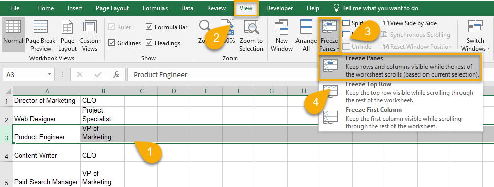
1. Select the third row, immediately below the two rows you wish to freeze in place.
2. Navigate to the View tab.
3. Click on the Freeze Panes option.
4. Select Freeze Panes from the drop-down menu.
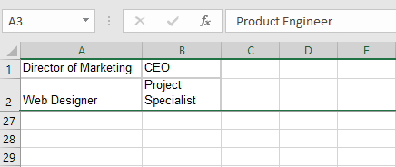
Voila! If you try to scroll down your spreadsheet, you will find that the top two rows are now frozen in place and will stay at the top of your document.
Why Do You Need to Freeze Rows?
If you have a large spreadsheet in Excel, you can freeze the top rows of your document to make working with your data so much easier.
There are a few benefits to freezing rows in Excel. First, it allows you to keep important data visible at the top of your spreadsheet while you scroll down. This is especially useful to keep track of what each column represents.
Second, freezing rows can make it easier to work with large spreadsheets by helping you keep your place while you’re working so you don’t have to keep scrolling up and down the document.
Finally, freezing rows can make it easier to print your spreadsheet. If you have a lot of data in your spreadsheet, it can be hard to fit everything onto one page when you print it. Freezing rows can help you ensure that all of the important information is visible on your printout right where you need it.
