In Excel, the Concatenate function allows you to join together two or more strings of text into a single cell. This function is reversible.
To reverse the Concatenate function in Excel, click on the cell where you want to see the result and enter the following formula:
=TRIM(MID(SUBSTITUTE($A2,”,”,REPT(” “,999)),COLUMNS($A:A)*999-998,999))
In this formula, A2 is the cell with the combined text. Press the Enter key and drag the cell with its result to the right to make all the other values appear.
Quick Jump
Toggle3 Ways to Reverse the Concatenate Function in Excel
When you reverse the Concatenate function in Excel, you end up splitting one cell into several cells. This can be useful when you want to unmerge data from one cell.
Here we provide three distinct approaches to this task. Let’s take a closer look at each method.
Method 1: How to Reverse the Concatenate Function in Excel Using a Formula
1. Click on the cell where you want the result.
2. Go to the Formula bar and type the following formula:
=TRIM(MID(SUBSTITUTE($A2,”,”,REPT(” “,999)),COLUMNS($A:A)*999-998,999))
A2 is the cell containing the text you need to split.

3. Press the Enter key on your keyboard.
4. Drag the cell with the formula to the right so the other values appear in their own cells.

And there you go! You have split the text from one cell into multiple cells.
NOTE: This only works if the data is separated by commas.
Method 2: How to Reverse the Concatenate Function in Excel with the Text-to-Columns Option
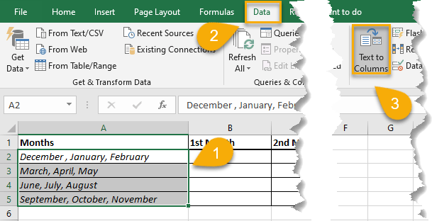
1. Select the data you need to split into multiple cells.
2. Navigate to the Data tab.
3. Pick the Text to Columns option.
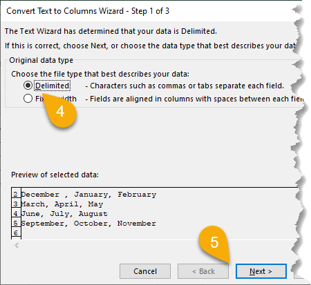
4. Choose Delimited as the file type that best describes your data.
5. Click Next.
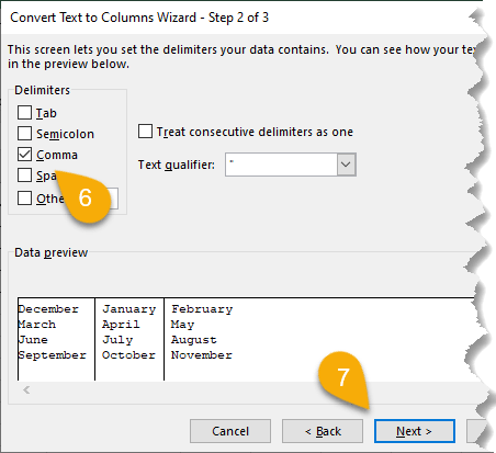
6. Mark the Comma Delimiter to remove commas from the rows and separate your data. The commas are used to tell the program where to separate the data.
7. Click Next.
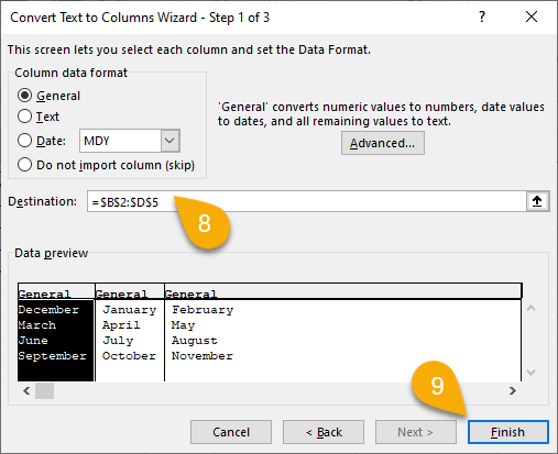
8. Write the Destination for your data. Here we set a destination of =$B$2:$D$5, where B2:D5 is the range of cells where we want the result to go.
If you prefer, you can also right-click and drag the cursor over the cells on the spreadsheet to select the range.
9. Click Finish.
10. Confirm your action by selecting OK.

Voila! You’ve successfully done it!

Method 3: How to Split Text Using the Flash Fill Option in Excel
1. To split the text in the first cell (A2), click on the cell where you wish to start the split (B2) and enter the first word manually.

2. Click and drag from the bottom right corner of that cell to the right until the other cells are filled with their values.

It’s very easy! To apply this function to each row, simply repeat the process.

Here is our result!
NOTE: This only works for lists that Excel can extrapolate on its own, such as a list of months or days or numbers in order.
Reversing the Concatenate Function in Excel FAQs
What is the Opposite of Concatenation?
The opposite function of the Concatenation function splits a text into parts rather than joining them together into one long row. This could be useful in certain situations where you need to manipulate or extract specific data from a row of text.
What Are Some Uses for Reversing the Concatenate Function in Excel?
Reversing the Concatenate function in Excel could help you separate names into first and last name columns, separate address information into multiple cells, or create a list of items from a single cell.
What Are the Benefits of Reversing the Concatenate Function in Excel?
There are several benefits to using the opposite function of concatenate in Excel:
- Save Time: It can save you time by reducing the number of steps you need to take to unmerge data.
- Better Manipulation and Analysis of Your Data: If you have a list of names in one cell, you can use the reverse of concatenation to split them into first and last name columns. This can be helpful for sorting or filtering your data.
- Avoid Mistakes: It can help you avoid the errors that can occur when unmerging data manually.