
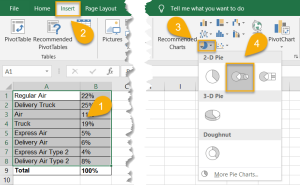
To create a Pie of Pie Chart in Excel, highlight your data and go to the Insert menu. Next, in the Chart submenu, select Insert Pie or Doughnut Chart, and choose the Pie of Pie Chart.
To learn more, check out the detailed description below where you will see how to create a Pie of Pie Chart, format the data in this chart, and change the chart style quickly and easily!
How to Add a Pie of Pie Chart
Start off by following the chart creation method as described below.
- Select your data.
- Navigate to the Insert menu.
- In the Chart submenu, click on Insert Pie or Doughnut Chart.
- Pick the Pie of Pie Chart type.
Voila! With those few steps, you have added a Pie of Pie Chart to your worksheet.

How to Format the Data in a Pie of Pie Chart
Creating a chart is the easiest part of the process. In order to improve your chart, follow the instructions below to make your chart unique.
Chart Title
Add a title to your chart that tells the reader exactly what content is contained within it. Here is how you can do that:
- Double-click on the title you want to change.
- Enter the name you prefer.

- Press the Enter key on your keyboard.
Easy as ABC! Let’s move on!
Data Labels
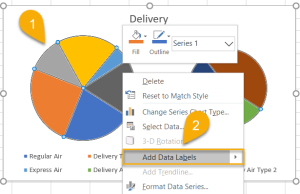
Data Labels is a feature in Excel that allows you to add labels to data points in your chart. You can use data labels to show the value of each data point as well as the percentage of the total each data point represents. Let’s take a look at how to add data points to your chart.
- Right-click on the chart.
- Select the Add Data Labels option.
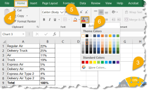
If you want the labels to be more visually appealing, you can change their color as well.
- Select the labels.
- Go to the Home menu.
- Navigate to the Font section and click on the Font Color option.
- Choose a color that works best for your chart. Be sure to make it visible against the chart and any background color you may have.
A piece of cake!
How to Change the Chart Style
If you want to change the appearance of your chart but don’t have time to play around with the options available, you can apply a preset style to it to help it stand out. To do this, follow these simple steps.
- Click on the chart.
- In the Design menu, look through the styles available and choose the best style for your worksheet.

If you do have some time and would like to personalize your chart even more, here are some ways to help add detail:
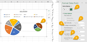
- Click on the chart.
- Select the Series Option from the Format Data Point menu.
- Choose the values you need to show on your chart.
- Pick the number of second plot values.
- Set the Point Explosion.
- Change the Gap Width.
- Choose the Second Plot Size.
Play with the values to determine what looks best to you.
Pie of Pie Chart Free Template
Grab our free Pie of Pie Chart Excel template to practice with your data.

Pie of Pie Chart in Excel FAQs
If you still have questions, check out the following FAQs!
What is a Pie of Pie Chart?
A Pie of Pie Chart is a type of chart that allows you to display data in a more efficient way. This method is especially useful when your data set has a lot of small values that are difficult to see on a regular Pie Chart. With this chart, you can break down a larger section of the primary pie chart into smaller pieces with the secondary pie.
What are the use cases of a Pie of Pie Chart?
The Pie of Pie Chart is typically used when there are a few large values in a data set and many small values. You can compare the relative sizes of other values more easily by breaking out the largest values into a separate pie chart.
