
We deal with data every day, and the more data we deal with, the more we need to find a way to organize it effectively. Google Sheets provides a free option for many of us to create and format spreadsheets for our data, but we often come across problems that leave us scratching our heads.
When working in a program like Google Sheets, it doesn’t take much for problems to arise due to incorrect formatting or incomplete formulas. This plagues experienced users and newbies alike.
In this article, we will dive into the topic of how to apply conditional formatting to cells, such as cell color, based on the data in another cell. This can help you avoid easy mistakes as you work in Google Sheets.
Sample Data
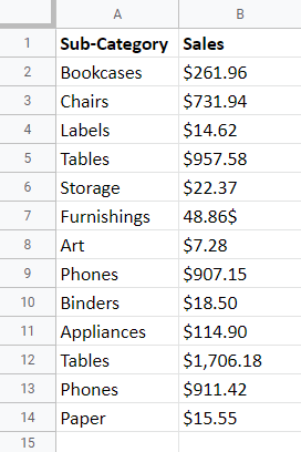
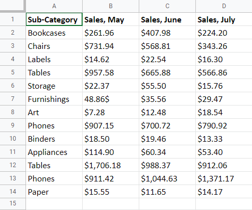
To start off with, let’s use the following dataset as an example, where column A contains a list of sub-categories and column B displays the sales value for each.
How to Apply Conditional Formatting Based on Other Cells
Conditional formatting can help you draw attention to crucial information in your dataset at a glance. Let’s see what we need to do to get that set up.
How to Highlight Cells with Conditional Formatting Based on the Value in Another Cell
1. Select the column containing the sub-categories (A2:A14).
2. Navigate to the Format tab.
3. Choose the Conditional formatting option.
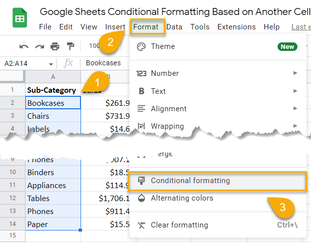
The Conditional format rules task pane will appear.
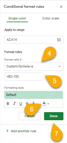
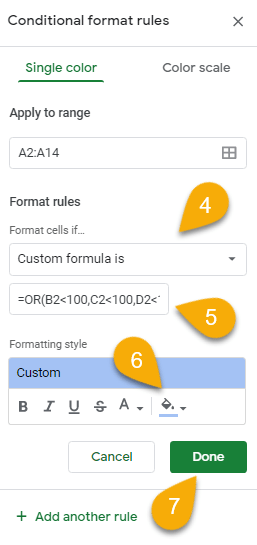
4. Choose the Custom formula is option under the Format cells if… format rule.
5. Next, type the formula =B2<100, where…
- B2 is the cell with the price value.
- 100 is the value specified in the condition.
6. Under Formatting style, select the fill color to apply a highlight to the cell.
7. Click Done when finished.
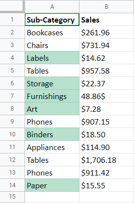
Easy peasy! Now any cell with a value less than 100 will be highlighted.
How to Highlight Cells with Conditional Formatting Based on the Values in Multiple Other Cells
Suppose you have a dataset as shown below, and you want to highlight cells in one column based on the values in the other columns.
Let’s see how to apply the conditional formatting based on the values of multiple other cells.
1. As before, highlight the cells containing the sub-categories (A2:A14).
2. Next, go to the Format tab.
3. Click on the Conditional formatting option.
4. Pick the Custom formula is option under the Format cells if… format rule.
5. Next, type the formula =OR(B2<100, C2<100, D2<100), where…
- B2, C2, and D2 are the columns with the price values.
- 100 is the value specified in the condition.
6. Under Formatting style, select the fill color to apply a highlight to the cell.
7. Select Done when finished.
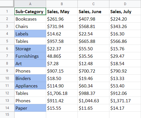
Voila! Now the cells will change color if all the conditions are met.
Conditional Formatting FAQ
Occasionally, we may be perplexed by the number of options available in Google Sheets. Users frequently search for answers to queries about conditional formatting. Read on to learn a bit more yourself.
What Does Conditional Formatting Mean?
Conditional formatting in Google Sheets is an amazing tool that allows you to apply formatting options to cells based on the values in other cells.
This is incredibly useful when you want to highlight certain cells based on whether or not they meet certain criteria. For example, you could use conditional formatting to highlight all the cells in a column that are greater than 100.
You may still encounter problems when creating conditional formatting rules if the cells in your sheet are not formatted correctly. For example, if you want to format a cell based on the numerical value in another cell, the first cell must be formatted as a number. If it is not, the conditional formatting rule will not work.
You also need to make sure you use the correct formula. Don’t miss a math sign or add another one, as this could also result in the condition not being met.
How to Use Conditional Formatting for Dates
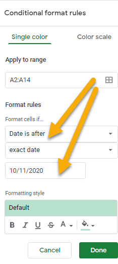
You can also use conditional formatting on cells that contain dates, not just numbers. Use the same formatting algorithm suggested above, but change the conditions in the Conditional format rules panel to apply the Date is, Date is before, or Date is after format rule, then type the appropriate date.
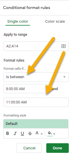
How to Use Conditional Formatting for Time
As with the previous example, setting up conditional formatting in relation to time involves establishing a condition based on date. The difference here is that you must select the Is between format option and establish the range for the time period required.
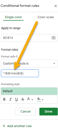
How to Use Conditional Formatting Based on the Lowest and Highest Value
There are times when we may need to find a specific value. In Google Sheets, we can limit and highlight these values by using conditional formatting based on the lowest and highest value. To do this, set up the custom formula =B:B=max(B:B) and/or =B:B=min(B:B) (where B is the name of the column) in the custom formula box of the Format rules panel. You may need to select Add another rule if you wish to apply both. Format the cell color as with the other conditions. This will highlight certain values within the range indicated.
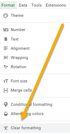
How to Remove Conditional Formatting
Sometimes you may have conditional formatting applied to certain cells, and you want to remove the formatting. Thankfully, this is an extremely simple process. Simply select the data and click Clear formatting from the Format menu.
In this article, you have learned how to apply conditional formatting to cells in your Google Sheets spreadsheet in order to highlight specific information within your dataset. This is especially useful when working with large datasets and wanting to discern the data at a glance. Try it out for yourself and see how it can help you work with your data more efficiently.
