To create and use Filter Views in Google Sheets, highlight your data, go to the Data menu, click on the Filter views option, and select Create new filter view. Next, tap on the Filter icon, check or uncheck the options you need to personalize your filter, and press OK.
Read on below to learn more about how to create a Filter View in Google Sheets in an easy and convenient way. This article will teach you how to use, save, share, and delete the Filter View. So, let’s get down to business!
Quick Jump
What Is a Filter View?
A Filter View is a way to save your filter settings in Google Sheets. With this feature, you can quickly apply your custom filters without having to set it up every time.
Filter Views can be useful if you regularly need to filter your data in different ways. For example, you could create a Filter View for each month’s data or for data that meets certain criteria.
What’s the Purpose of Filter Views in Google Sheets?
Filter Views in Google Sheets offer a way to view, manipulate, and analyze data stored in a spreadsheet without actually changing the underlying data.
This is useful for Google Sheets users who are dealing with the same data but who need to be able to make their own edits and changes to the data without disturbing others. This means that other users won’t be able to see the changes you’ve made, and you can easily work with your edits. It allows different team members to focus on different aspects of the data.
How to Create a Filter View in Google Sheets
Check out the step-by-step guide below to learn how to create a Filter View in seconds:
- Select the data.
- Navigate to the Data menu.
- Choose the Filter views option.
- Pick Create new filter view.
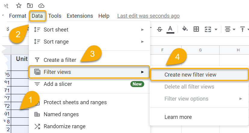
Easy-peasy! That’s all it takes to create a new Filter View.
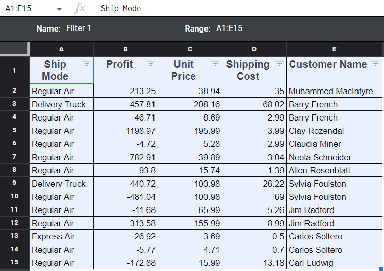
Next, let’s learn how to use and modify it!
- Click on the Filter icon.
- Check or uncheck the options you need or experiment with the other actions available.
- Hit OK.
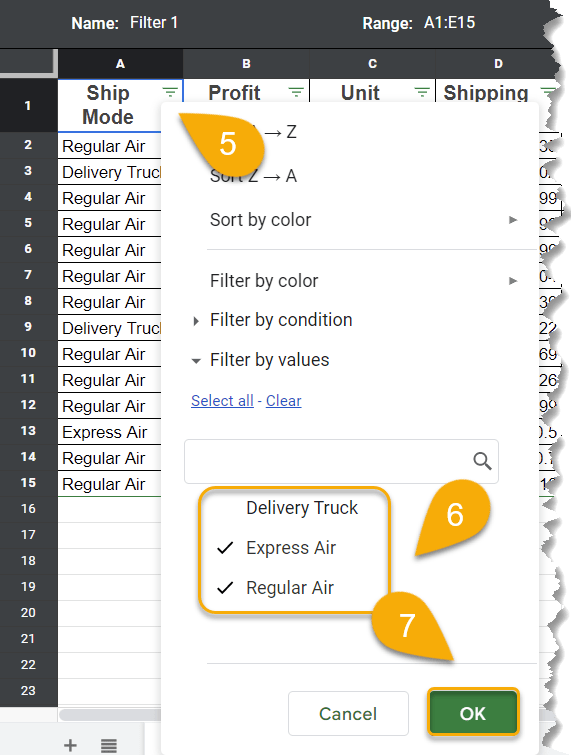
That’s it!
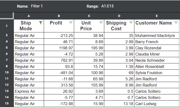
How to Save a Filter View for Reuse
Once you’ve made changes in data using the filter, it’s saved automatically. But if you want to display the edited data in the list, take the following steps:
- Click on the Name box and enter a name for the filter.
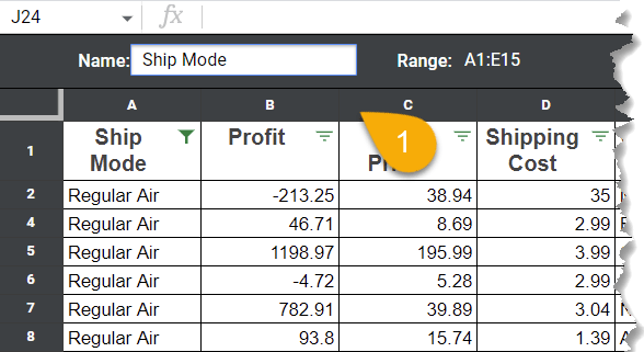
- Next, simply press the Enter key on your keyboard.
Easy as ABC!
How to Find Your Saved Filter Views
If you want to use one of your previously saved Filter Views, take a look at this step-by-step guide on how to find them and apply them:
- Go to the Data menu.
- Choose the Filter views option.
- Select the filter you need.
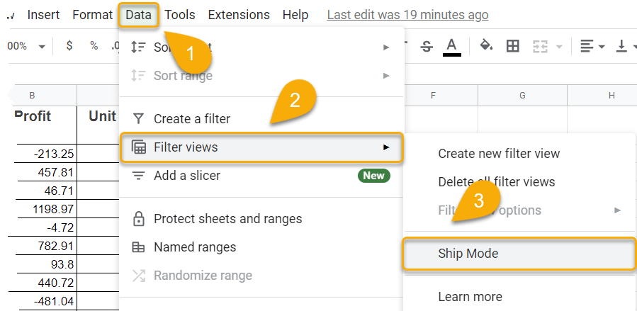
Voila! It’s that simple.
How to Share a Filter View with Others
If you want to share your Filter View with colleagues or friends, just do the following:
- After applying the Filter View, select the URL for your document.
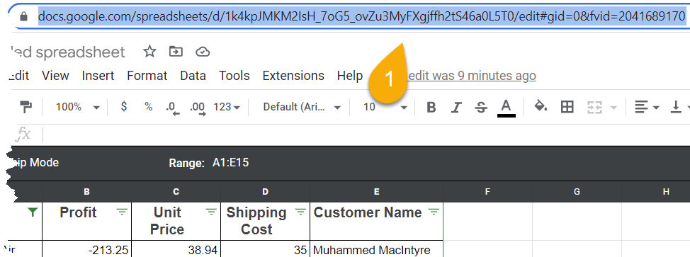
- Press the Ctrl + C (Windows) / Cmd + C (Mac OS) key combination to copy it.
- Share the document with other users by hitting the Ctrl + V / Cmd + V keys to paste it in a message to them.
That’s all it takes.
How to Delete a Filter View
Use the method below if you want to revert the document back to its original state:
- Navigate to the Data menu.
- Choose Filter views.
- Select Filter view options.
- Click Delete.
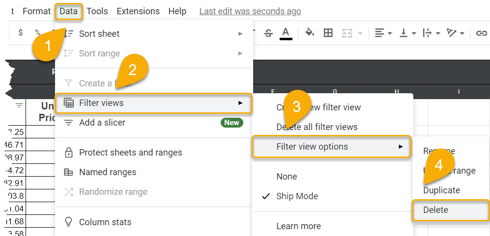
That’s it! The filter will be removed.
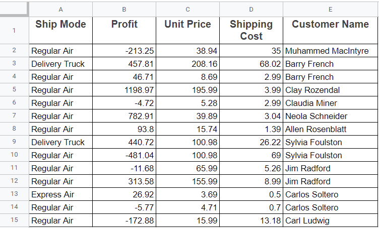
Can you lock a Filter View in Google Sheets?
Yes, you can lock a Filter View in Google Sheets. Here’s how you do it:
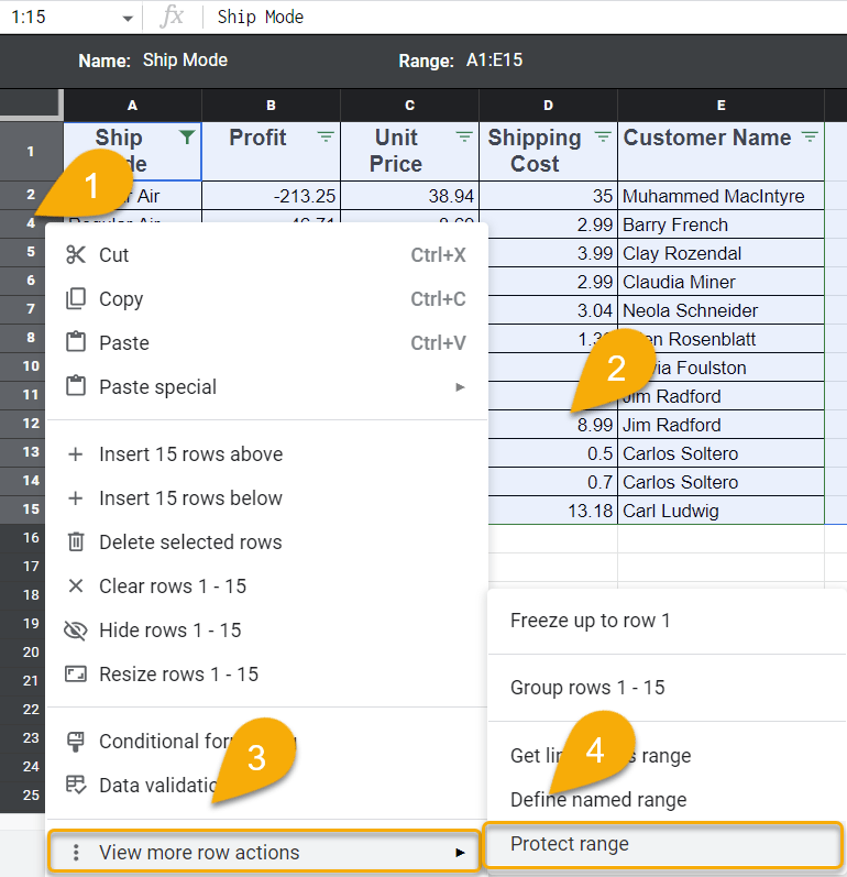
- Select the range you need to protect.
- Right-click on it.
- Choose View more row actions.
- Pick Protect range.
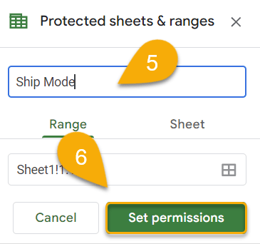
- Enter a description for the highlighted section.
- Click on the Set permissions button.
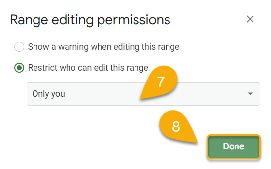
- Select the user(s) who can edit this range.
- Tap Done.
Congratulations! You have done it!