To lock a row in Google Sheets, click on the top-left corner of the worksheet and drag the cursor down to lock a row into place.
In this article, you will learn a couple methods on how to lock a row in Google Sheets without much trouble. Scroll down to learn more!
Quick Jump
ToggleMethod 1: Using the Mouse
This is the easiest way to lock a row in Google Sheets (also known as freezing the row).
Difficulty: Beginner
Time Estimate: 2 Seconds
1. In the top-left corner of the sheet where the column and row headers meet, click and hold the bottom border of the corner cell. (It will highlight in blue when selected.)
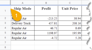
2. Drag the cursor downward to lock the row.
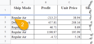
Super easy! You have successfully locked the row in place. (Note: You can pull it down further to lock more than one row.)

Method 2: Using the View Menu
This method uses the toolbar to lock rows in place. Check out the steps below to learn how it’s done.
Difficulty: Beginner
Time Estimate: 5 Seconds
1. Go to the View menu.
2. Select the Freeze option.
3. Choose the number of rows you need to lock into place.
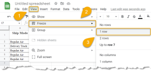
Just like that, it’s done!

Locking Rows in Google Sheets FAQs
The FAQ below will provide you with more information on the topic of locking rows in Google Sheets.
How do I lock rows in Google Sheets for sorting?
To lock rows for sorting, you just need to select the rows that you want to lock, click the Data menu, and choose the Create a filter option.
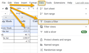
Then click on the top-left corner of the sheet and drag the cursor down to lock rows as needed (as described above).
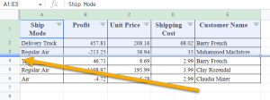
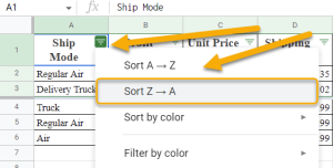
Click on the Filter icon and set the filter you need.
How do I lock a cell in Google Sheets so it can’t be edited?
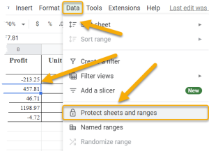
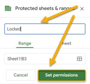
To lock a cell so it can’t be edited, highlight the cell(s) you want to lock then click on the Data menu and select Protect sheets and ranges.
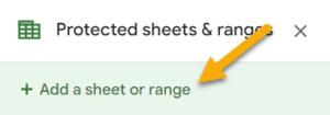
In the new menu that pops up, select Add a sheet or range.
Next, enter the description (whether it’s a sheet or a range of cells) and hit the Set permissions button.
How do I lock cell references in Google Sheets for my formula?
The process of locking cell references in Google Sheets is pretty simple. Simply click on the cell where you need your formula, go to the Formula bar, enter the formula, click on the cell reference included in the formula, press F4 on your keyboard to add the dollar sign automatically (this locks the reference to that particular cell), and hit Enter.

The cell reference for your formula has now been locked into place so it won’t change if you copy the formula into a new cell.