To multiply in Google Sheets, select a cell, go to the Formula bar, type the values for the equation with the asterisk symbol between them, and press Enter.
In this article, we will look at three strategies for multiplying your values quickly and simply. Keep reading to see which one works best for you.
Quick Jump
ToggleMethod 1: Using the Asterisk Sign
Difficulty: Beginner
Time Estimate: 5 Seconds
1. Select the cell where you need to get the result.
2. Go to the Formula bar and type the values you wish to multiply with the asterisk symbol between them. In our example, we use =34*12.
3. Press the Enter key on your keyboard.

Easy as ABC! Let’s move on!
Method 2: Using Cell References
Difficulty: Beginner
Time Estimate: 5 Seconds
1. Choose the cell where you want your result.
2. In the Formula bar, enter the formula =A1*B1, where A1 and B1 are cells with your values.
3. Hit the Enter key.

Voila! The calculation is complete.
Method 3: Using Formulas
Difficulty: Beginner
Time Estimate: 10 Seconds
1. Click on the cell where your answer should be.
2. Navigate to the Formula bar and type the formula =MULTIPLY(34,12). In our example, the values being multiplied are 34 and 12. Enter the values you need.
3. Press Enter.

And there you go!
Multiplying in Google Sheets FAQs
Check out some of these FAQs for a greater grasp on this subject!
How do I multiply one column by another in Google Sheets?
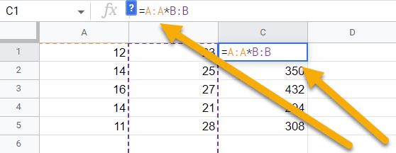
To multiply one column by another, start by selecting the cell where you want your result. Then go to the Formula bar, enter the formula =A:A*B:B, and press Enter. A:A and B:B are the ranges of the columns you want to multiply. Here is the result:

How do I multiply cells in different worksheets?
To multiply cells in different worksheets, select the cell where you want your result, go to the Formula bar, type the formula =Sheet2!A1*Sheet1!A1, and press the Enter key. In our case, A1 is the reference cell in both Sheet1 and Sheet2.
