Removing duplicates in Google Sheets is a function that allows you to find and remove duplicate values in your data. This can be useful if you have a large dataset and want to clean it up, or if you want to make sure that there are no duplicates in your data before you perform any further analysis.
Trying to remove duplicate data in a dataset in Google Sheets can be a daunting task if you try to do it manually. Large quantities of data can be overwhelming, and visually recognizing the same items may not be simple.
In this article, we will learn how to remove duplicate values in Google Sheets quickly and easily.
Quick Jump
ToggleSample Data
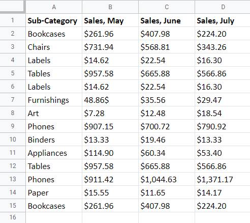
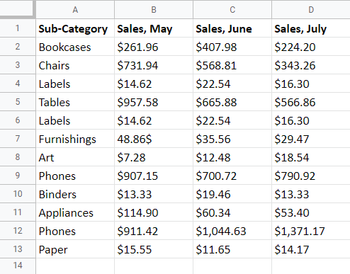
Let’s start with the sample data below, which has subcategories in column A and sales indicators in columns B, C, and D.
5 Ways to Remove Duplicates in Google Sheets
Google Sheets offers several different ways to remove duplicates in your dataset. Pick the method that works best for you. Let’s get down to business!
How to Remove Duplicates in Google Sheets with the Remove Duplicates Tool
1. Select the data where you need duplicates removed (A1:D15).
2. Go to the Data tab.
3. Click on the Data cleanup option.
4. Choose Remove duplicates.
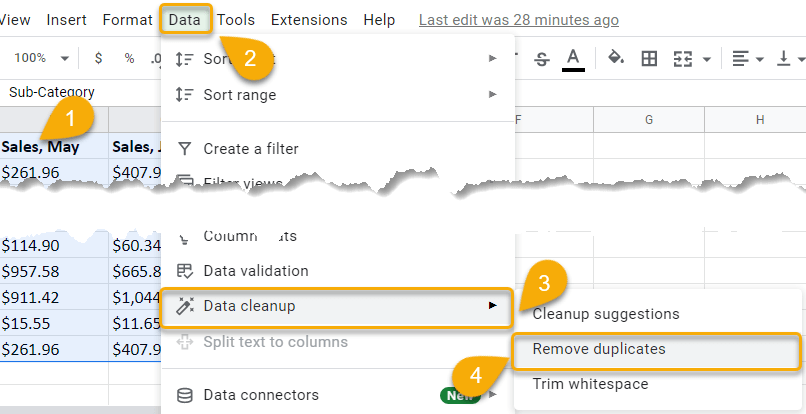
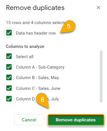
5. Add a checkmark beside each column where you want duplicates removed.
6. Click Remove duplicates.
7. Finally, click OK.
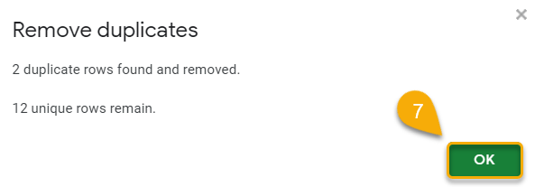
Easy as ABC! The duplicates have been swiftly eliminated.
How to Remove Duplicates in Google Sheets with Formulas
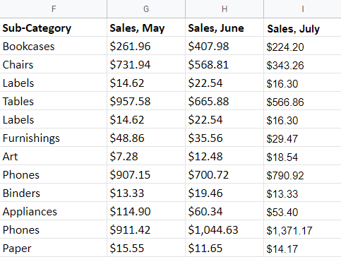
This method is slightly different in that it does not remove the duplicate values. Rather, it creates a new dataset with the duplicates removed, so you end up with two datasets: the original and the one without the duplicates.
Formula 1
1. Click on the cell where you want the new dataset to start.
2. Type the formula =UNIQUE(A1:D15) in the Formula bar, where (A1:D15) is the range with the data we need.
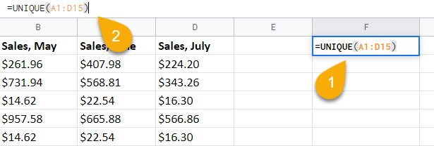
3. Press the Enter key on your keyboard.
Formula 2
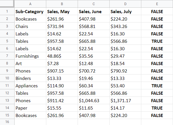
The following formula labels each row as TRUE or FALSE depending on the values in a particular column, thus helping you find duplicates.
1. Choose the cell where you need to insert the data.
2. Type the formula =COUNTIF(B$2:B2,B2)>1 in the Formula bar, where B is the column with the values you need to check.
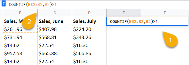
3. Again, on your keyboard, press the Enter key.
Formula 3
1. Pick the cell where you want the new dataset to start.
2. Type the formula =ArrayFormula(UNIQUE(TRIM(A1:D15))) in the Formula bar, where (A1:D15) is the range with the data we want to review for duplicates.

3. Hit the Enter key on your keyboard.
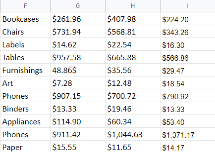
You’ve done it!
How to Remove Duplicates in Google Sheets with Conditional Formatting
1. Highlight the cells with the values you want to review for duplicates (A1:D15).
2. Navigate to the Format tab.
3. Click on the Conditional formatting… option.
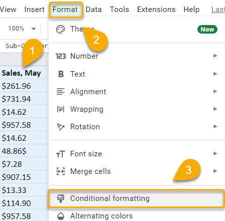
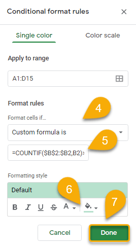
4. Under Format rules, for Format cells if…, select the format rule Custom formula is.
5. Type the formula =COUNTIF($B$2:$B2,B2)>1.
6. Choose a color in the Formatting style section to highlight any duplicates.
7. Hit Done.
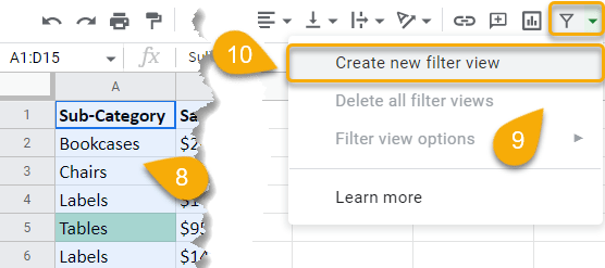
8. Select the data (A1:D15).
9. Go to the Filter views button and click on the little arrow to the side to reveal the drop-down menu.
10. Choose Create new filter view.
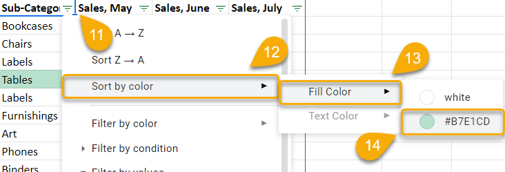
11. Click the Filter icon in the header row.
12. Pick the Sort by color option.
13. Select Fill Color.
14. Choose the color you selected to highlight duplicates.
15. Select the rows with the duplicates that appear at the top of the list.

16. Right-click the selected rows and select Delete selected rows to remove the rows from your dataset.

There you go! You have removed the duplicates.
For a better understanding of how to use this feature, check out our guide on using conditional formatting based on another cell in Google Sheets.
How to Remove Duplicates in Google Sheets with Pivot Tables
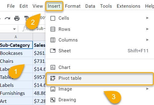
1. Select your dataset (A1:D15).
2. Navigate to the Insert menu.
3. Choose the Pivot Table option.
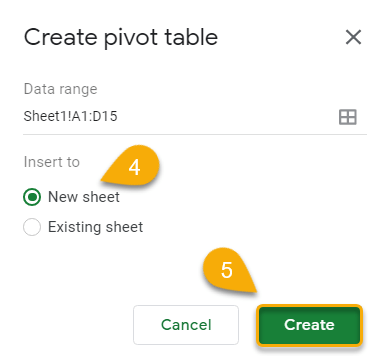
4. Pick the sheet where you want to insert the data.
5. Click Create.
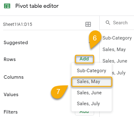
6. Hit the Add button to add rows to the table.
7. Pick the row or rows you need (here we use all the rows).
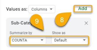
8. In the Pivot table editor, go to the Values tab.
9. Add each column to the Values tab. Under Summarize by, select COUNT, and under Show as, select Default. Do this for each one.
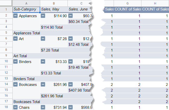
That’s it! Here you can see the number of duplicates—each item that has a number greater than 1 beside it.
How to Remove Duplicates in Google Sheets with Add-ons
Before removing duplicates in this way, you need to install the add-on.
1. Go to the Extensions menu.
2. Choose the Add-ons option.
3. Pick Get add-ons.

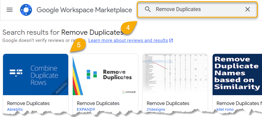
4. In the Search box, type Remove Duplicates.
5. Choose the required add-on.
6. Click the Install tab.

7. Hit Continue.

8. Choose an account to continue to install the Remove Duplicates add-on.
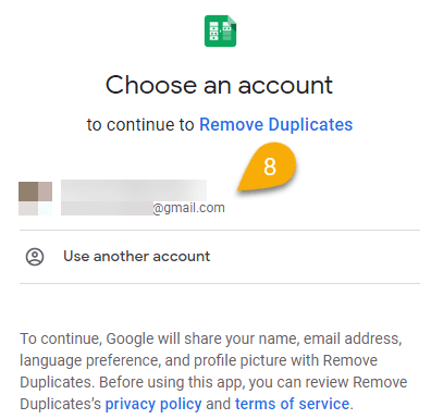
9. Confirm the installation and click Allow.

Now that the application is installed…
10. Select your dataset (A1:D15).
11. Navigate to the Extension menu.
12. Click the Add-ons option.
13. Pick View document add-ons.
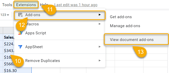
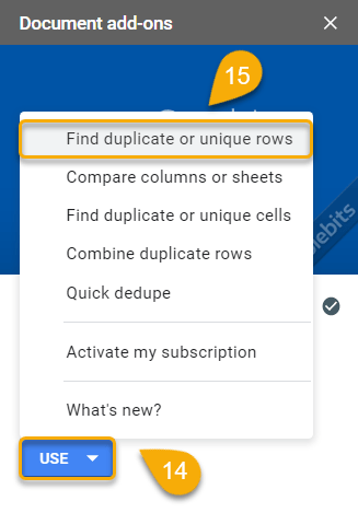
14. Click the Use button on the Document add-ons menu.
15. Choose Find duplicate or unique rows.
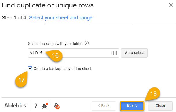
16. Type the range of your data (A1:D15).
17. Check the option to create a backup copy of the sheet.
18. Hit the Next button.
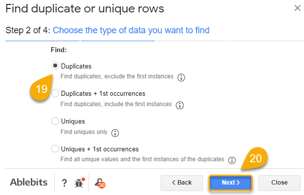
19. Under Find, select Duplicates.
20. Click Next.
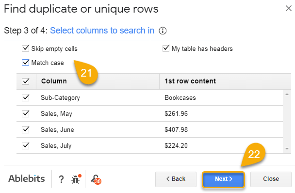
21. Select the columns to search by adding checkmarks beside each one.
22. Again, click Next.
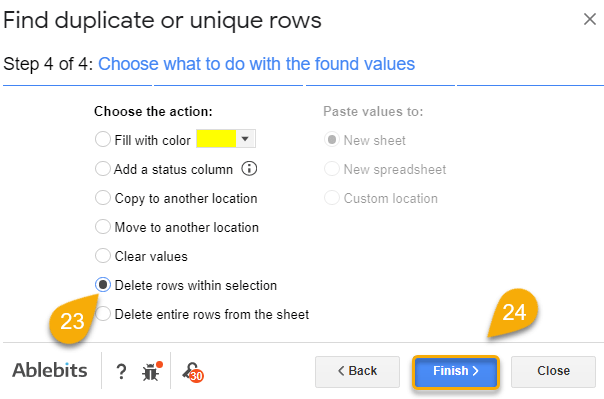
23. Pick Delete rows within selection.
24. Hit Finish.
And here is the result!

There are a few different ways to remove duplicates in Google Sheets. The most common way is to use the Remove Duplicates tool, which can be found under the Data tab. Alternatively, you can use the Unique function through the use of formulas, apply Conditional Formatting in combination with the Filter function, set up a Pivot Table, or use a specific add-on to help you find the duplicates in your data.
Whichever method you choose, make sure you understand how it works before you apply it to your data to make sure you don’t accidentally delete important information.