Underlining is an easy and effective way to draw attention to important data, data which you want your reader to notice. Google Sheets offers a number of ways you can underline the data in your spreadsheet.
With the proper use of this tool, you can greatly enhance your document in very little time. In this post, we will go through various ways to underline, the underline types, and some specific underline use cases in Google Sheets.
How to Underline All Text Within a Cell
Underlining all text within a cell in Google Sheets is very simple.
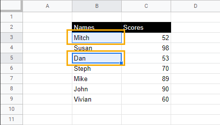
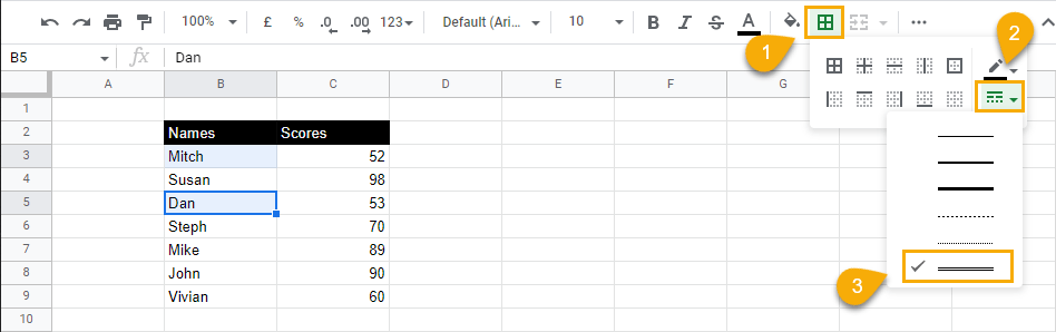
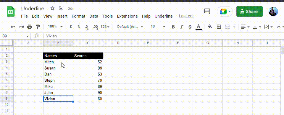
The sample data below contains a list of scores and their corresponding names. Let’s say you want to identify the people with scores less than 60 using an underline. Here are the steps to do so:
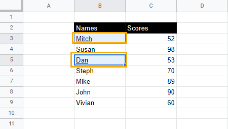
1. Identify the cells with scores less than 60 (Mitch and Dan). Press and hold the Ctrl key to select both cells.
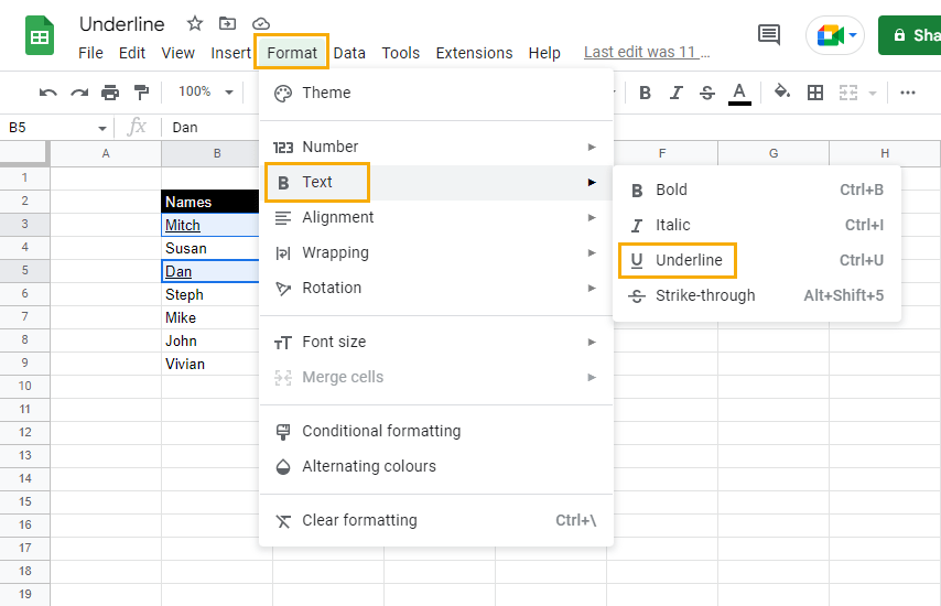
2. Go to the Format menu, select Text, and click on Underline. Alternatively, use the keyboard shortcut Ctrl + U for Windows or Cmd + U for Mac to underline the selected cells.
How to Underline Part of the Text Within a Cell
To underline part of a text within a cell, the process is slightly different from underlining the whole thing.
Using the sample data from the previous section, we can underline parts of the names as follow:
1. Double-click on the cell you want to underline.
2. Select the letters or characters you want to underline.
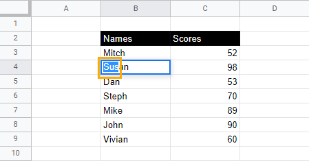
3. Use the keyboard shortcut Ctrl + U (Cmd + U) to underline the selected text.
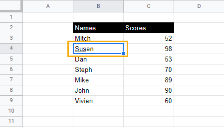
Underlining just part of the text must be done within the cell itself. Using the underline command from the Format menu will always underline the entire text.
Unfortunately, this does mean that for every cell where only part of the text is underlined, it will have to be done cell by cell.
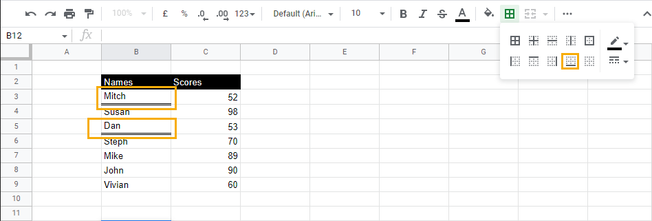
How to Underline an Entire Cell
Underlining an entire cell is a bit different from underlining all the text within a cell. When you underline an entire cell, you are, essentially, creating a bottom border to the cell.
To underline an entire cell in Google Sheets, follow these steps:
1. Select the cells you want to underline.
2. In the toolbar options, select Borders and choose the Bottom border option.
This will add an underline or a bottom border to the entire cell.

How to Double Underline an Entire Cell
To double underline in Google Sheets, simply take the previous underline style (underlining an entire cell) a step further, as the double underline is actually a border style.
Follow these steps to double underline:
1. Select the cells you want to double underline.
2. In the toolbar options, under the Borders menu, select the Border style drop-down and choose the double line option.
3. Select Bottom border to apply it to the cells.
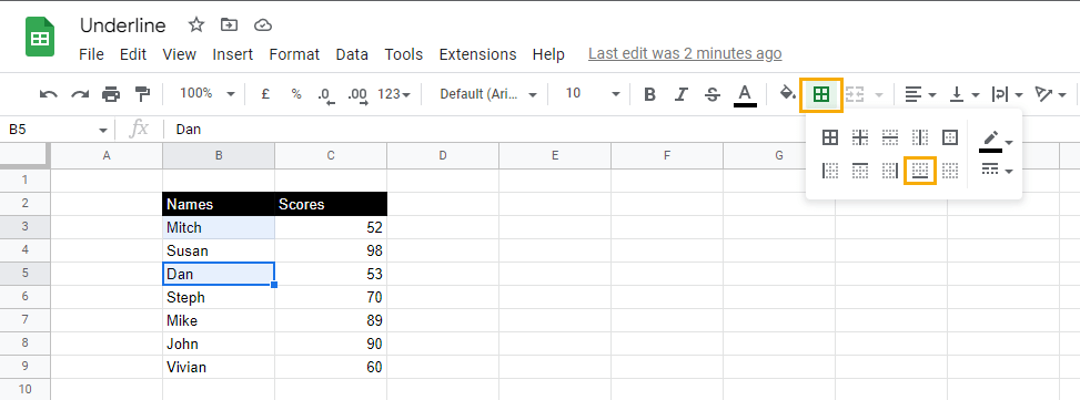
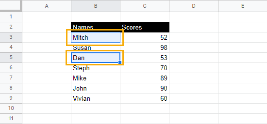
How to Underline a Row
Say we want to separate the highest scores from the lowest scores using a row underline as a divider. Here’s how to do it:
1. Identify the row you want to underline and select the row number to highlight the entire row.
2. While keeping the row selected, go to the toolbar menu, select Borders, and choose the Bottom border option.
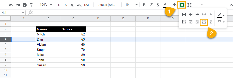
When you do this, a thick dark line will appear from the beginning of the row on the right across to the other side of the spreadsheet.
How to Create a Dotted Underline
To create a dotted underline, just modify the border style on your cell or row. Google Sheets provides a range of border styles which you can use for various situations.
Simply follow these steps:
1. Select the cells or row you want to underline.
2. Go to the toolbar options, select Borders, and click on the Border style drop-down menu. Choose the dotted line.
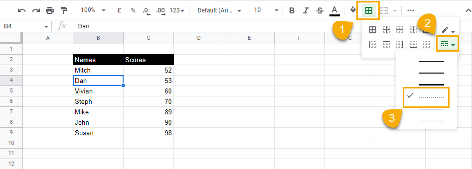
3. Select the Bottom border option to apply the border to your selection.
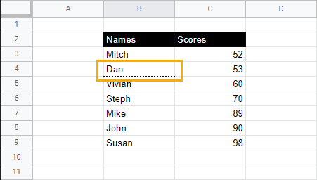
You can also modify a previously underlined cell or row. Just select the underlined row or cell and follow step two.
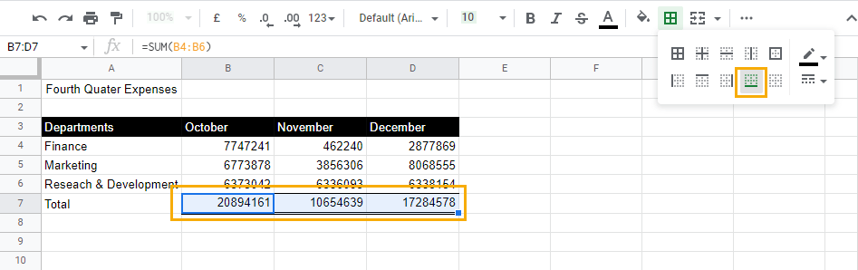
How to Set Up Accounting Underline for Totals in Google Sheets
To set up accounting underlining for totals in Google Sheets, you only need to add a single-line top border and a double-line bottom border to the Total rows.
Follow these steps to create an accounting underline for totals:
1. Select the cells where you want to add an accounting underline.
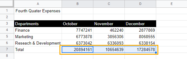
2. While keeping the cells selected, go to the toolbar and select Borders. Then click on the Top border option to apply a top border to these cells.
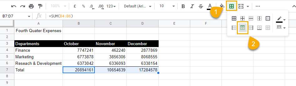
3. Still keeping the rows selected, go to the Border styles drop-down menu and select the double lines.
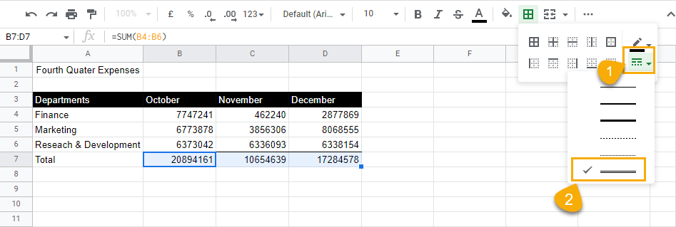
4. Select the Bottom border option to apply this double line to the bottom of the cells.
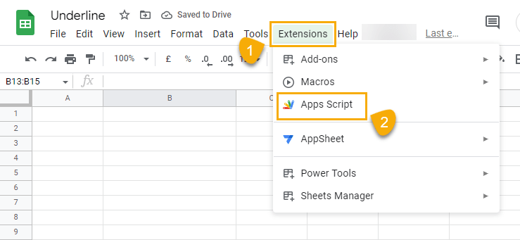
How to Underline Cell Text Using Apps Script
Adding an underline to individual cells can involve many clicks and mouse movements, not to mention taking time. With an Apps Script, you can simplify this process.
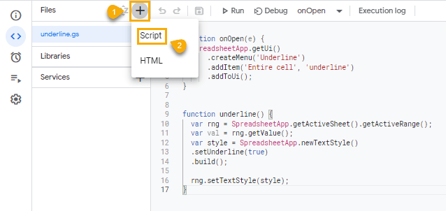
To create an Apps Script, go to the Extensions menu and select Apps script. This will open the editor window where you can create an Apps Script.
When the Apps Script editor opens, copy and paste the syntax below.
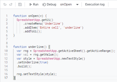
function onOpen(e) {
SpreadsheetApp.getUi()
.createMenu(‘Underline’)
.addItem(‘Entire cell’, ‘underline’)
.addToUi();
}
function underline() {
var rng = SpreadsheetApp.getActiveSheet().getActiveRange();
var val = rng.getValue();
var style = SpreadsheetApp.newTextStyle()
.setUnderline(true)
.build();
rng.setTextStyle(style);
}
The syntax contains two functions. Each one is explained below.
function onOpen(e) {
SpreadsheetApp.getUi()
.createMenu(‘Underline’)
.addItem(‘Entire cell’, ‘underline’)
.addToUi();
}
function onOpen(e) { }: This first line of code creates and names the function. The function parameter is a keyword that creates the function. The function syntax is as follows
function <function-name> ( ) {//code to be executed}
With this syntax, the function keyword serves as the building block for a custom function or menu.
In this function, the onOpen(e) parameter names the function. However, onOpen(e) is also a trigger.
Triggers are keywords that allow functions to run automatically when certain events happen. The onOpen(e) trigger runs the function when you open or reload the spreadsheet. All subsequent lines of code are contained within the curly brackets.
SpreadsheetApp.getUi(): This code gets the user interface of the currently active spreadsheet.
.createMenu(‘Underline’): The createMenu() function is a method under the SpreadsheetApp class that creates a new menu in the active spreadsheet.
The parentheses is where you enter the name for the new menu being created. For the createMenu method, characters in the parentheses must be enclosed in quotation marks. Here, the new menu is called Underline
.addItem(‘Entire cell, ‘underline’): This method adds a new item to the newly created menu. It takes two parameters in its parentheses. The first parameter — ‘Entire cell’ — provides a name for the new item while the second parameter — ‘underline’ — references the name of the function that will run on the new item that is selected.
.addToUi(): This method doesn’t take any arguments. It simply adds the newly created menu to the active spreadsheet’s interface.
Summarily, the first function creates the custom menu.
function underline() {
var rng = SpreadsheetApp.getActiveSheet().getActiveRange();
var val = rng.getValue();
var style = SpreadsheetApp.newTextStyle()
.setUnderline(true)
.build();
rng.setTextStyle(style);
}
function underline: As in the first function, this code names and creates the function.
var rng = SpreadsheetApp.getActiveSheet().getActiveRange(): When this syntax runs, it will return the selected range in the active spreadsheet and store it in the rng variable.
This is made possible because the SpreadsheetApp keyword tells the script to run on the currently active spreadsheet. The getActiveSheet() method returns the currently open sheet in the spreadsheet and the getActiveRange() method returns the selected cell or range in the currently active sheet.
var val = rng.getValue(): This syntax creates the val variable and then uses the getValue() method to return the values of the ranges stored in the rng variable.
var style = SpreadsheetApp.newTextStyle(): The style variable is used to store the textstyle builder created using the newTextStyle() method.
Imagine the textstyle builder as a template. In it, you can create or add any type of textstyle formatting you want. The methods that follow this syntax add the text formatting.
.setUnderline(true): This adds an underline format to the textstyle builder. It takes a boolean argument — true or false. When set to true, it adds an underline formatting.
.build(): This method locks in all the changes applied to the textstyle builder. Essentially, the build() method signifies that you’re done creating a template for the textstyle being built.
rng.setTextstyle(style): This syntax applies the styles stored in the style variable to the ranges stored in the rng variable using the setTextStyle() method.
The setTextStyle() method applies a textstyle to a value or range. It takes one argument which points to the textstyle one wishes to apply. Here, the textstyle has already been created and stored in the style variable, hence, the reason why it appears as the parameter in the setTextStyle parentheses.
After you copy and paste this syntax in the Apps Script editor, make sure you hit the Save and Run commands.
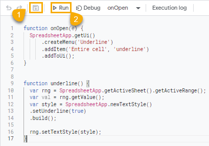
When you’re done, refresh your spreadsheet. The new custom menu will appear named Underline. To use it, follow these steps.
1. Select the range you wish to add the underline format.
2. Click on Underline, then Entire cell.
Underlining in Google Sheets: FAQs
Is there a shortcut to the underline button in Google Sheets?
Yes, there is a shortcut to the underline button. The Ctrl + U (Cmd + U) keyboard shortcut will underline all the text in a selected cell.
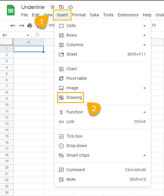
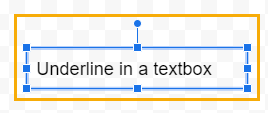
Can I underline a textbox in Google Sheets?
Yes. You can underline characters in a textbox. To underline in a textbox, follow these steps:
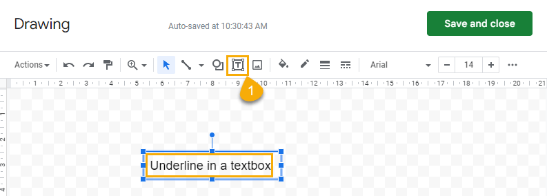
Insert a textbox by going to the Insert menu and clicking on Drawing.
Click on the textbox icon and enter the text you want to underline.
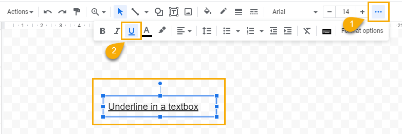
To underline all text in a textbox:
1. Select the textbox.
2. Click on the ellipses on the right side of the toolbar and select the underline icon. You can also use the underline shortcut Ctrl + U (Cmd + U).
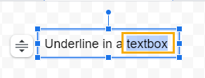
To underline some of the text in a textbox:
1. Double-click inside the textbox and select the characters you want to underline.
2. Underline the selected character using the underline command from the ellipses menu or the keyboard shortcut.
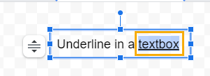
When you’re done and after you’ve hit the Save and Close option, the textbox will be inserted into the spreadsheet with the characters underlined.
Is there a Google Sheet function to underline text?
Google Sheets doesn’t have an underline function.
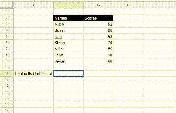
How do I count the number of cells with an underline?
There’s no Google Sheets function for counting the number of cells with an underline. To count the number of cells with an underline, you will need to create a custom function using Apps Script.
Use the first step in the earlier Underline custom menu to open the Apps Script editor window, then follow these steps to create the custom function:
1. Add a new script by clicking on the plus “+” icon and selecting Script from the options.
2. Rename the newly created script, then copy and paste the syntax below.
function COUNTUNDERLINE(range) {
var currRange = SpreadsheetApp.getActiveRange();
var currSheet = currRange.getSheet();
var currFormula = currRange.getFormula();
var input = currFormula.replace(/.COUNTUNDERLINE\(/gi, ”).replace(/\).*/gi, ”);
var range = currSheet.getRange(input);
var styles = range.getTextStyles();
var underline = []
for (var i = 0; i < styles.length ; i++) {
for (var j = 0; j < styles[0].length ; j++) {
var cellsUnderlined = styles[i][j].isUnderline();
if (
cellsUnderlined == true
) {
var count = [0];
underline.push(count)
}
}
}
return underline.length
};
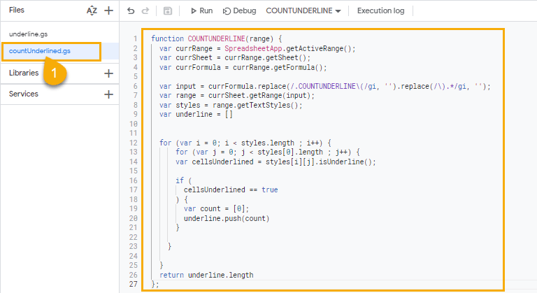
The script creates a custom function that you can use just like regular Google Sheets. The custom function, COUNTUNDERLINE, will return the number of underlined cells in a range.
Here’s how each line in the syntax works:
- function COUNTUNDERLINE(range) { }: This first line of code creates and names the function using the “function” keyword. The syntax of the “function” keyword is as follows:
function <function-name> ( ) { //code to be executed };
Using this syntax, the “function” keyword defines this Apps Script. The <function-name> parameter is where you define the function’s name. Here, we name the function COUNTUNDERLINE.
The bracket that follows the <function-name> parameter is used to define a variable as the input for the custom function. Custom functions can be designed to take values or not, like the Underline function created earlier.
When a custom function is designed to receive input values, the input values (or arguments) are specified in the parentheses beside the <function-name> parameter.
The number of arguments or input values a custom function will have is determine the number of variables you will create. When a custom function has more than one argument, each will be separated by a comma.
The COUNTUNDERLINE function will only take one argument, which is the cell ranges that may or may not be underlined. These cell ranges will be stored in the range variable.
Every other line of code will go into the {//code to be executed} parameter.
- var currRange = SpreadsheetApp.getActiveRange(): This syntax returns the currently selected cell or range and stores it in the currRange variable.
- var currSheet = currRange.getSheet(): This syntax returns the currently active sheet and stores it in the currSheet variable.
- var currFormula = currRange.getFormula(): The getFormula() method returns the formula in the present cell. Since the currRange variable holds the currently selected range or cell, getFormula() then returns the formula in that cell and stores this value in the currFormula variable.
The first part of this syntax returns the custom function as a string. That is, assuming we have entered the custom function =COUNTUNDERLINE(A1:A5) in cell B7, this first part of the formula will return =COUNTUNDERLINE(A1:A5) as text.
From this illustration, B7 will be the active range that the currRange variable will return, and the currFormula variable will return =COUNTUNDERLINE(A1:A5) as text.
In the next part of the syntax, we will extract the range from the text value returned and use it to get the underlined cells in the range.
- var input = currFormula.replace(/.COUNTUNDERLINE\(/gi, ”).replace(/\).*/gi, ”): This syntax searches for and removes everything from =COUNTUNDERLINE(A1:A5) except for the range A1:A5. To achieve this, the syntax uses the replace() method.
The replace() method is a string method with the syntax replace(searchChar, newChar). The searchChar parameter refers to the character to be replaced in the string, while the newChar refers to the character that will replace the searchChar.
In this syntax, replace() uses a regular expression to remove the searchChar parameters. The first replace() removes the “=COUNTUNDERLINE” and replaces it with blanks. The second replace() removes the “)” and also replaces it with blanks.
This leaves the range A1:A5 which is stored in the input variable.
- var range = currSheet.getRange(input): This syntax uses the getRange() method to get the specific range stored in the input variable. This value is stored in the range variable.
This step must be carried out because the range stored in the input variable is in text format and doesn’t point to any particular range in the spreadsheet.
However, in the range variable, this text value is used to point to a specific cell range in the spreadsheet.
- var styles = range.getTextStyles(): getTextStyles() returns a two-dimensional array of the textstyles in a range. In this case, it returns, in a two-dimensional array, the textstyles of the cell ranges in the styles variable.
- var underline = [ ]: This creates an array that is stored in the underline variable.
This part of the syntax gets the textstyle of the range. The textstyle is stored in a two-dimensional array. To reference these textstyles, we need to loop through each textstyle in the array. For this, we used the for loop.
A loop lets you run the same code over using different values, and there are different types. In this code, we use the for loop to go through the entire textstyles stored in the styles variable.
The for loop has the following syntax:
for (statement 1; statement 2; statement 3) { // code block to run }
The statement 1 parameter runs just once, statement 2 sets the condition for executing the code block, and statement 3 runs every time the code block is executed. The statement 2 parameter determines when the loop ends. When the condition in the statement 2 parameter is false or not met, the code block stops and the loop ends.
for (var i = 0; i < styles.length ; i++) {
for (var j = 0; j < styles[0].length ; j++) {
var cellsUnderlined = styles[i][j].isUnderline();
if (
cellsUnderlined == true
) {
var count = [0];
underline.push(count)
}
}
}
In this for loop statement, a variable i is created and equated to zero. i < styles.length means that i will be less than the length of the number of values in the styles variable. The styles variable holds in a two-dimensional array the textstyles collected from the range, so the length of styles will be equal to the number of textstyles in the array. That is, if there are 10 textstyles in the array, the length of styles will be 10. And var i will always be less than the number of textstyles in the array; that is, if styles.length = 10, i will range from 0 to 9.
i++ means that var i will continue to increase and stop once i is equal to or greater than styles.length.
Essentially, “var i = 0; j < styles. length; i++” translates into “create a variable i that is equal to zero and continue increasing the value of i, but stop when it is equal to or greater than the length of the styles array.”
A second for loop follows the first one: for (var j = 0; j < styles[0].length ; j++. This creates a new variable j, equates it to zero and increments it until it is equal to or greater than the length of styles[0].
Here, styles[0] references the first textstyle in the array. Values in an array can be called using their index numbers. Apps Script uses zero-based indexing, which means the first value in an array has an index of 0.
styles[0] references the first textstyle in the array. Since this is just one value, it has a length of 1. In the loop, this implies that j cannot be greater than or equal to 1, essentially setting its value to 0.
The reason for creating these two variables — i and j — is that we’re looping through a single-column two-dimensional array (styles). While var i will reference all row elements and keep changing, var j will reference the column element and remain static, hence, 0. With this configuration, it is possible to get all the textstyles from the array.
var cellsUnderlined = styles[i][j].isUnderline();
if (
cellsUnderlined == true
) {
var count = [0];
underline.push(count)
}
After setting the loop conditions, the code to be executed follows.
- var cellsUnderlined = styles[i][j].isUnderline(): This creates a variable cellsUnderlined. It checks if a particular textstyle from the styles array has an underline. The isUnderline() method returns true or false. Therefore, this code returns a true if a textstyle is underlined and false if it’s not.
Note that, here, i and j now assume numerical values. So styles[i[[j] translates to styles[0][0] (the textstyle in row index 0, column index 0). Since j will always be zero, only the value of i will change. And this will continue until the statement 2 parameter in the first for loop statement is unmet.
This way, every textstyle in the array can be checked for an underline. Whatever this block of code returns is stored in the cellsUnderlined variable.
- if (cellsUnderlined == true) {var count = [0]: This if statement checks if the cellsUnderlined variable returns true. Essentially, it picks out all the “trues” in the cellsUnderlined variable and stores them in a new variable: count.
In this code, for every true that exists in the cellsUnderlined variable, an array value “[0]” is added to the count variable.
- underline.push(count): push() is a method that adds items to an array. Earlier, we created an empty array and stored it in the underline variable. This code block adds every item in the count array to the underline array.
This marks the end of the for loop statement.
- return underline.length: The return keyword is used to instruct a function to produce a specific output. Here, the underline array now contains all the textstyles that are underlined. To know the number of underlined textstyles in the array, we simply count them using the length method.
This code block ensures that the function returns the number of cells in the range that are underlined.
Custom functions are case-sensitive. They also don’t have IntelliSense, so you must be careful of spelling and case errors when calling custom functions.
How do I troubleshoot Google Sheets not underlining text?
When you find that you can’t underline a cell in Google Sheets, the following reasons may be responsible:
- Edit permission not granted: if you’re not granted permission to edit a sheet or a range, you will not be able to underline. Check to see what kind of permissions you’re to which you’re privy.
- Error in custom underline function: If you’re using an Apps Script solution, check your code properly to ensure there are no errors.
- Blank cell: While you can add underline formatting to a blank cell, the underline will not be visible until the cell has additional characters. If you want to underline a blank cell, you will be better off adding bottom borders.
How do I remove an underline from hyperlinks in Google Sheets?
To remove the underline from hyperlinks, follow these steps:
1. Select the cell containing the hyperlink
2. Go to the Format menu, click on Text and select Underline. You can also use the Ctrl + U (Cmd + U) shortcut.
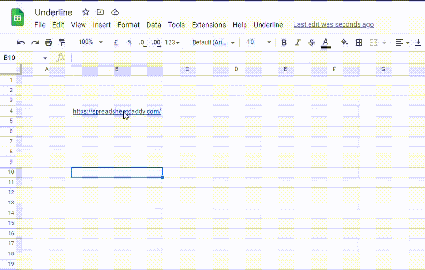
How do I copy and paste underline styling in Google Sheets?
To copy and paste underline styling in Google Sheets, follow these steps.
Assuming we want to apply the same underline style to the item in cell B10, here’s how to do it.
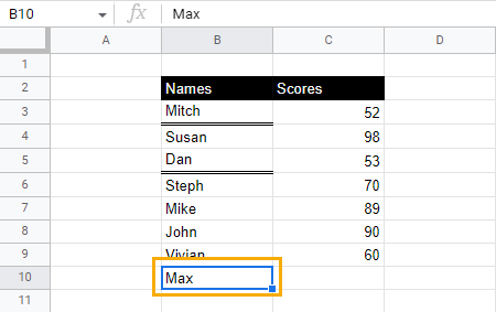
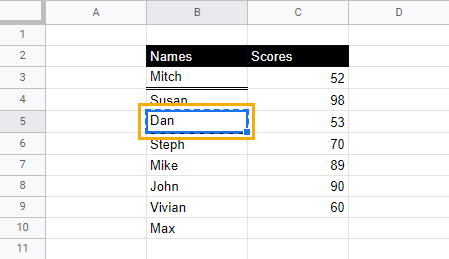
1. Select the cell with the underline style you want to copy. Press Ctrl + C (Cmd + C) to copy. After copying, the border around the cell should be blue and broken.
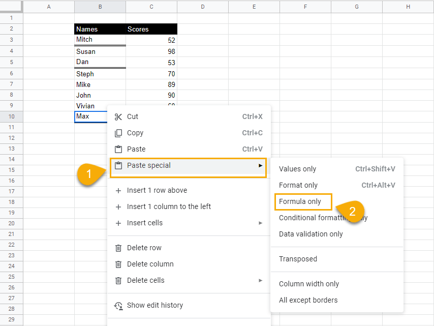
2. Select and right-click on the cell where you want to paste the underline format. From the drop-down menu, select Paste special and click on Format only.
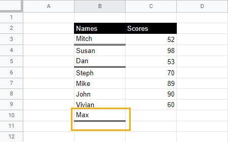
When you click away from the cell, cell B10 will now have the double underline.
Google Sheets underline formatting doesn’t show in a PDF file. What should I do?
If underline formatting doesn’t appear in a PDF file, go back to the sheet and reapply the underline format. Then export the PDF again.
Can I underline inside a comment in Google Sheets?
No, you cannot underline inside a comment in Google Sheets.
How do I underline spaces in Google Sheets?
You cannot underline a blank cell in Google Sheets. However, you can underline spaces.
Follow these steps:
1. Select a cell and double-click or press F2 to edit.
2. Using the spacebar, create the number of space characters you want inside the cell.
3. Use the Shift + Left arrow key to highlight the space characters.
4. Press Ctrl + U (Cmd + U) to add an underline.