To use the Does Not Equal operator in Google Sheets, select a blank cell, go to the Formula bar, enter the formula =A1<>”Apple” (“Apple” is simply an example text), and hit Enter. Lastly, drag the cell with the result downward to copy the formula for the rest of the list.
In order not to miss any important details about this topic, read through the article below. Here you will learn all about the Does Not Equal operator! Let’s take a look.
Quick Jump
How Do Comparison Operators Work in Google Sheets?
Google Sheets supports various comparison operators that allow you to compare two values and return a logical value (TRUE or FALSE).
Among the operators, the Equal (=) operator is one that gives a TRUE return if the two values being compared are the same.
The Does Not Equal operator in Google Sheets is represented by two inequality signs placed side by side (<>). This operator will return TRUE if the values on either side of it are not equal and FALSE if they are equal.
What Is the Does Not Equal Operator?
The Does Not Equal operator is a comparison operator that returns TRUE if the two operands are not equal to each other and FALSE if they are. For example, =2<>3 would return TRUE (because they are not equal), and =3<>3 would return FALSE (because they are equal).
This operator is most often used in conjunction with the IF function to create formulas that test for conditions that must be TRUE or FALSE.
Google Sheets Does Not Equal Operator: Syntax
The syntax of the Does Not Equal operator in Google Sheets is this:
=val1<>val2, where…
- val1 is your starting value.
- val2 represents the value you want to compare to the first value.
If you want to use the NE function instead, you can use the following formula:
=NE(val1, val2)
Here val1 and val2 are values you need to compare.
How to Use the Does Not Equal Operator (Real-World Example)
This section explains how to use the Does Not Equal operator step by step in order to obtain the result:
- Click on a blank cell.
- Go to the Formula bar and enter the formula =A1<>”Apple”, where A1 is the cell with the value, and Apple is your condition.
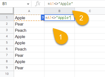
- Press the Enter key on your keyboard.
- Using the cell’s drag handle, you can apply the result to the rest of the cells in the list.’
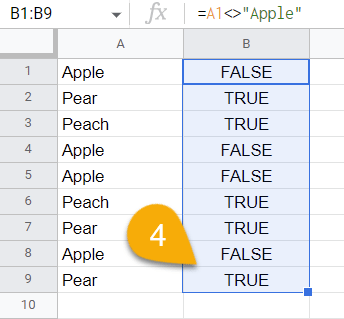
Voila! Just like that, you have done it!
Alternately, you can use the function NE as follows:
- Select the cell where you want the result.
- Navigate to the Formula bar and type the formula =NE(A1, B1). A1 and B1 are the cells with the values you need to compare.
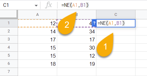
- Hit Enter.
- If you need to compare other values, drag the cell down to copy the formula through the rest of the list.
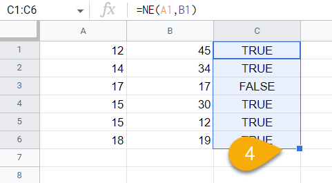
Super easy!
When Should You Use the Does Not Equal Operator?
The Does Not Equal operator can be used in a number of different situations. Here are a few examples:
- To test if two numbers are not equal to each other.
- To check if two cells contain different values.
- To compare two columns of data to see if they contain any mismatches.
- To find rows where a particular column does not contain a certain value.
Bonus: Using the Does Not Equal Operator with Conditional Formatting
This algorithm can be used in order to apply conditional formatting to certain values—such as a result of TRUE with a formula like the Does Not Equal operator. If you wish to do this, simply following these steps:
- Go to the Format menu.
- Pick the Conditional formatting option.
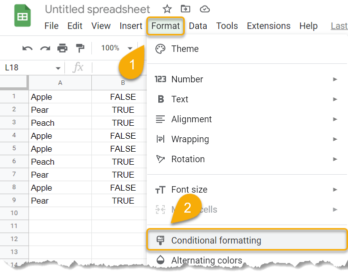
- Set the range of cells you want to apply this to.
- Under Format cells if…, choose Text contains.
- Enter the text you want to trigger a change in formatting (TRUE).
- Click Done.
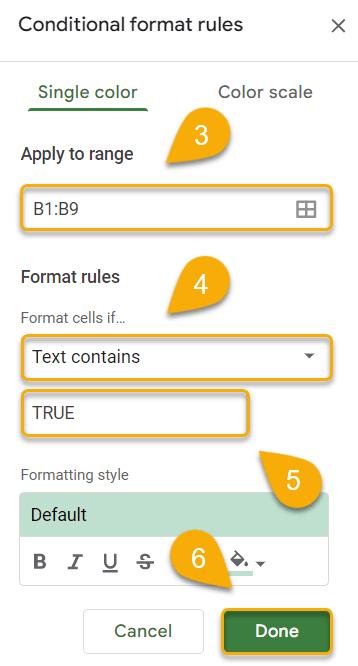
Easy as ABC! From the default settings, this will cause any cell with the result of TRUE to turn green.
Other Comparison Operators in Google Sheets
Google Sheets provides several other numeric operators that may apply to your document. Check out the list below for some of the most commonly used operators:
- Less than: <
- Greater than: >
- Equal to: =
- Less than or equal to: <=
- Greater than or equal to: >=