To make a pie of pie chart in Google Sheets, you need to create two separate pie charts and tie them together using a dashed line to show how they relate to each other since this chart type is not supported in Google Sheets.
Stick around to learn our workaround that doesn’t require AppsScript or add-ons. This article will show you how to display percentages of a small slice of a pie chart in Google Sheets.
Also, if you’re short on time, grab a copy of our free Google Sheets pie of pie chart template.
Step #1: Prepare Your Data
So, a typical pie of pie chart is made of two parts:
- The primary pie chart shows how the values in a data set compare against each other.
- The secondary pie chart breaks down a particular slice of the primary pie chart.
Because of that, a pie of pie chart allows for a more granular view of your data, making it possible to zero in on a certain slice of your primary pie chart to make data-driven decisions.
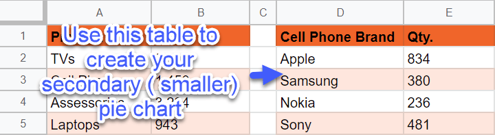
To illustrate the process from start to finish, we came up with this sample data table that showcases the sales figures of an electronics store.
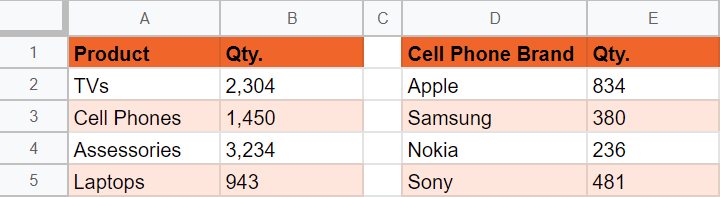
In our case, the first table (A1:B5) will be used to plot the primary pie chart whereas the second table (D1:E5) will be used to create the secondary pie chart dissecting the sales of cell phones by the brand.
So before we dive into the nitty-gritty, prep your data based on the table above so that you can easily retrace our steps.
Step #2: Create the Primary Pie Chart
Once we have our data all set up, it’s time to create the primary pie chart based on the first data table.
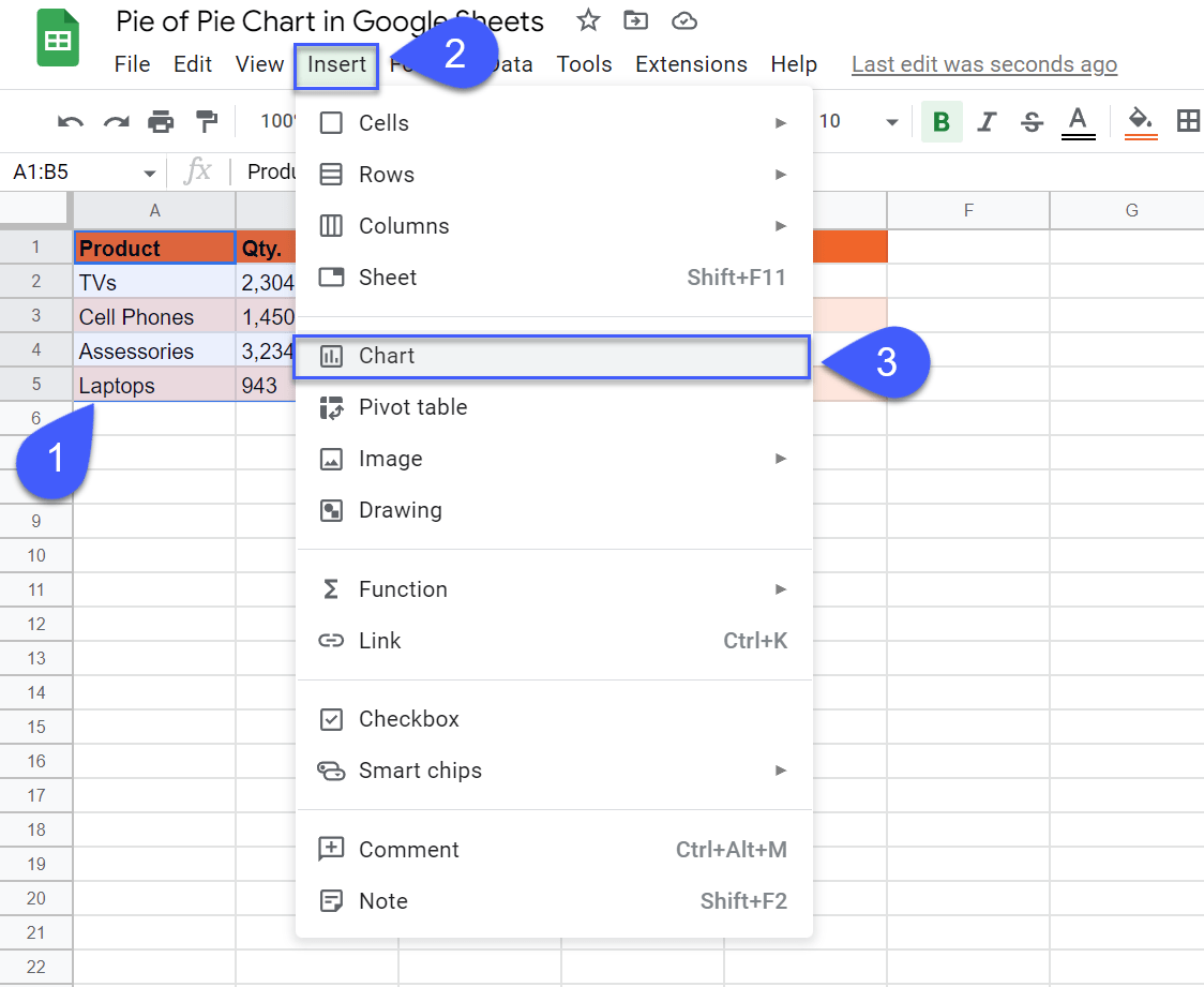
1. Highlight the first data table with the values for the primary pie chart (A1:B5).
2. Navigate to the Insert tab.
3. From the drop-down menu that appears, select “Chart.”
Once there, Google Sheets should automatically generate a regular pie chart. But if, for some reason, you get something else—it happens to the best of us—here’s what you need to do.
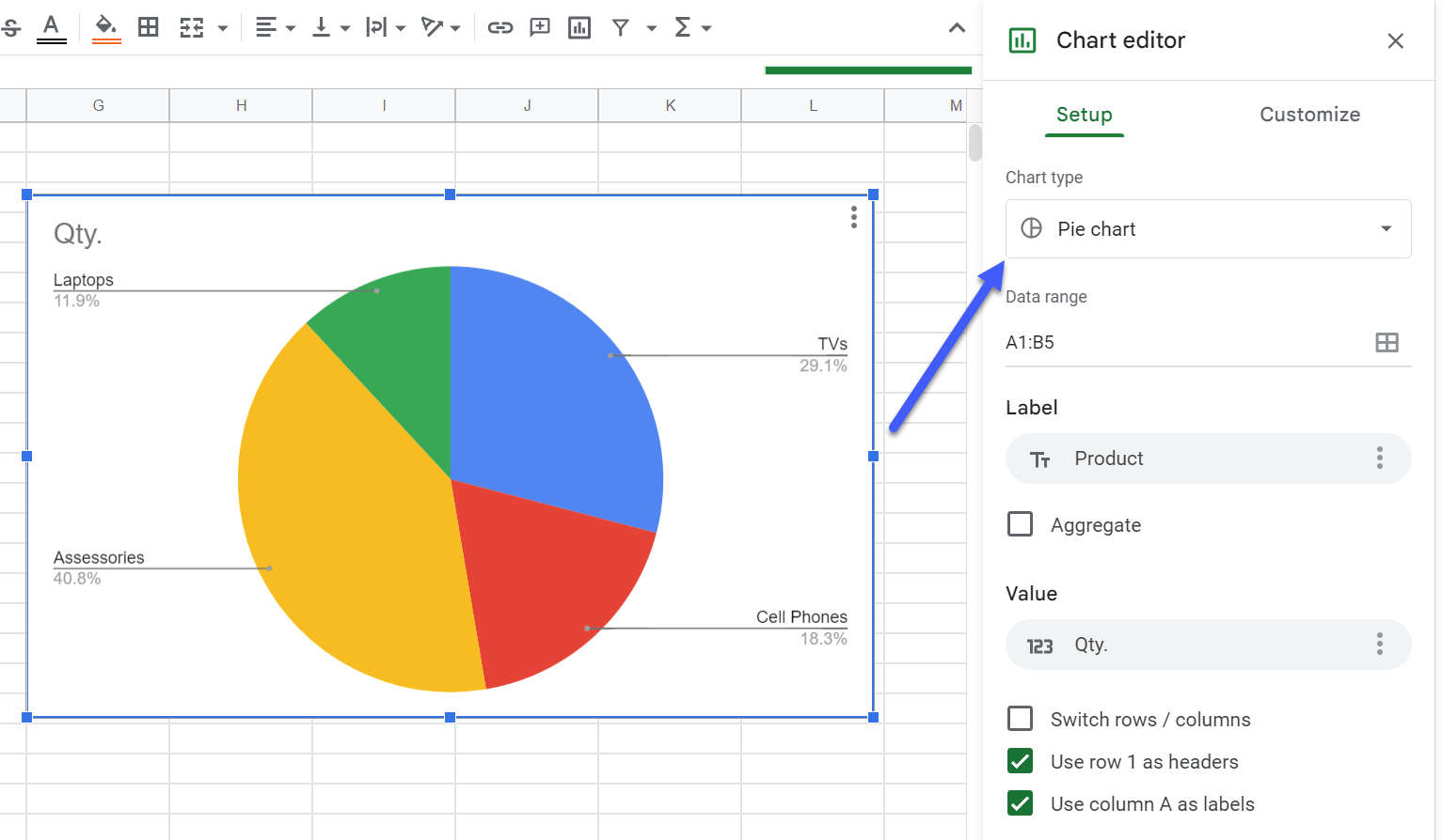
In the Chart editor task pane that pops up every time you create a new chart, navigate to the Setup tab. Under “Chart type,” click the drop-down menu and manually select “Pie chart.”
Now, it’s time to customize our primary chart to ensure that it looks nice and clean when we’re going to stack two pie charts on top of each other. Let’s start off with removing the chart border to seamlessly place two charts next to each other.
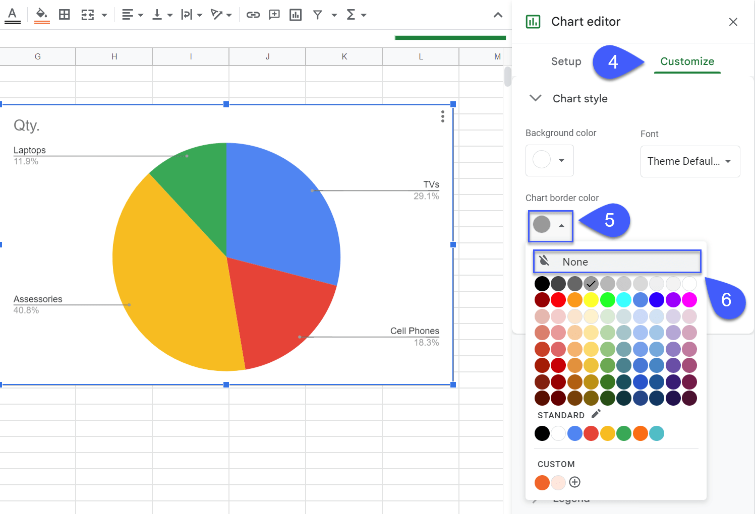
4. In the Chart editor, switch over to the Customize tab.
5. Hit the button under “Chart border color” to pull up the color palette.
6. Choose “None” to remove the border of your primary pie chart.
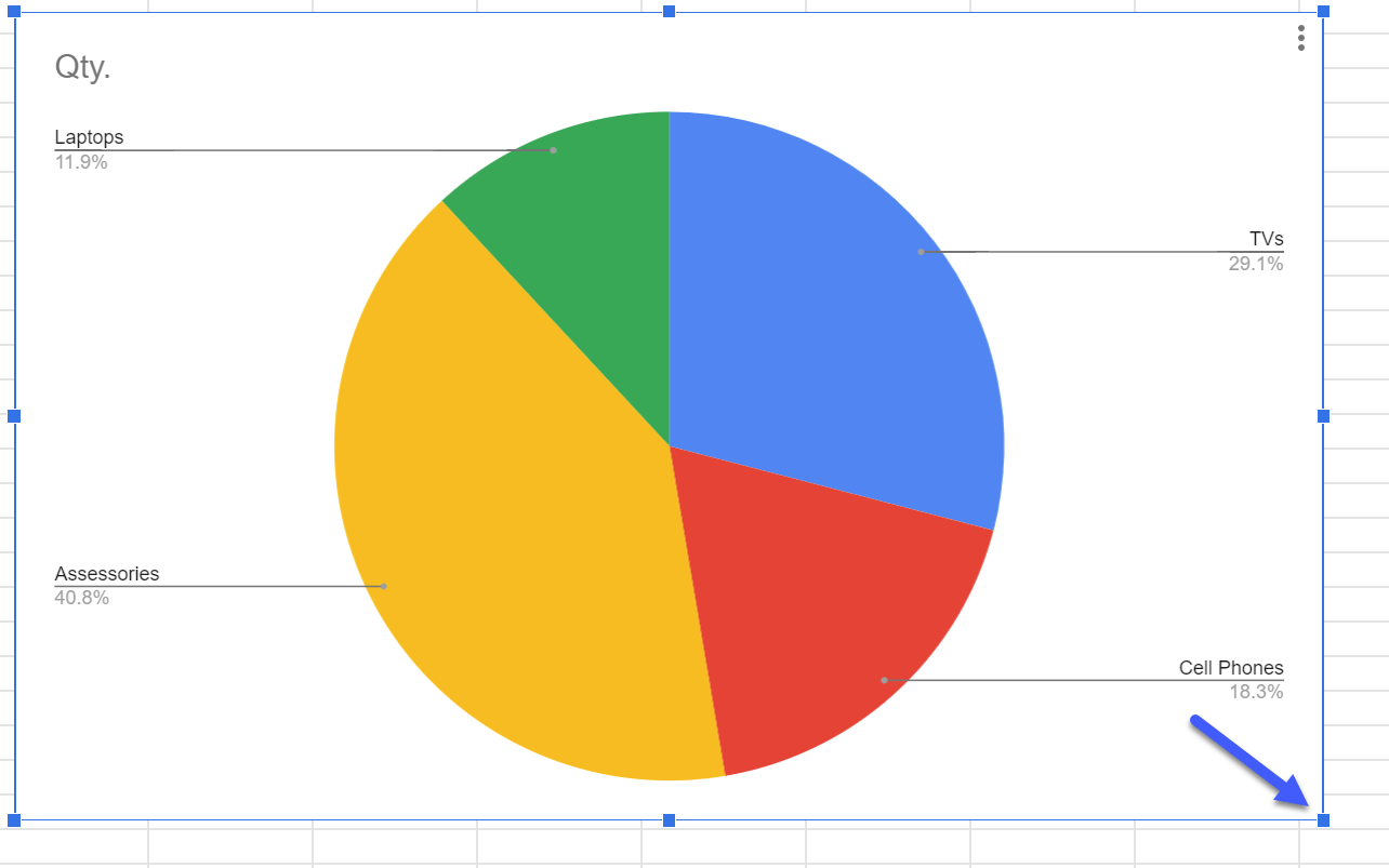
Next, we need to increase the chart area to fit two charts on one chart plot.
7. Drag the blue marker at the bottom left corner of the chart plot to increase the chart area.
Our next step is resizing the primary pie chart to free up some space for the secondary, smaller pie chart.
8. Double-click anywhere on the primary pie chart and resize it by dragging the white marker as shown below:
9. Finally, double-click on the chart title and change it to “Sales Q4 2022” to make it more descriptive.
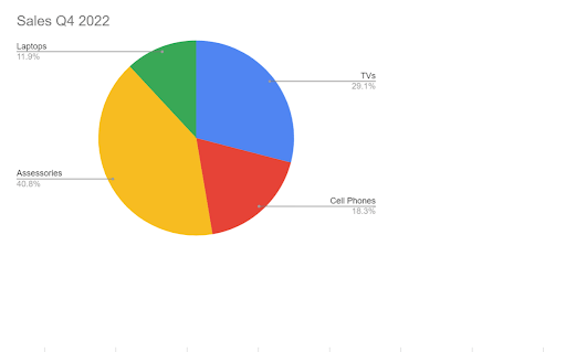
As a result, our primary pie chart is ready to go while the plot has enough space to fit the smaller pie chart we’re going to use to break down one of the slices of the main chart.
Step #3: Create the Secondary Pie Chart
The process of creating the secondary pie chart is very similar to the steps we covered above. The only difference is that we’ll need to remove the chart title to prevent text from overlapping.
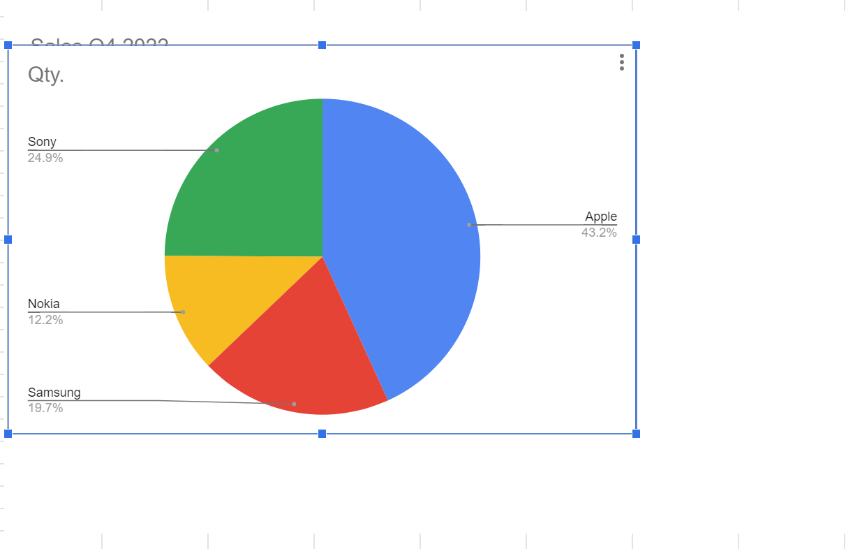
1. Create a regular pie chart from the second data table (D1:E5) by following the steps mapped out above (Highlight the second data table > Insert > Chart). If Google Sheets fails to generate the graph we need, in the Chart editor, change the chart type to “Pie chart.”
As a result, we get our second chart overlapping the primary one.
2. Remove the chart border by following Steps 4-6 in Section 1 where we did the same thing with the primary pie chart.
Here’s what our borderless chart looks like at this stage of the process:
 3. Now we need to delete the title of the secondary pie chart. Double-click on the chart title and press the Delete key.
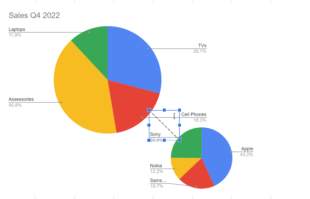
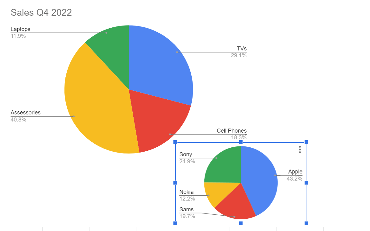
4. Finally, resize the secondary pie chart to make it fit the plot of the primary pie chart. Select the secondary pie chart, and drag the blue marker to make it smaller. Once there, place the secondary chart at the bottom left corner of the charting area.
As a result, your Google Sheets pie of pie chart should look this way:
Step #4: Add a Dashed Line to Illustrate Relationships Between Data
To add the final touches to our pie of pie chart in Google Sheets, we need to clearly demonstrate how the two graphs relate to each other.
There are multiple ways you can do that, but adding a simple dashed line is, arguably, the least time-consuming of all of them.
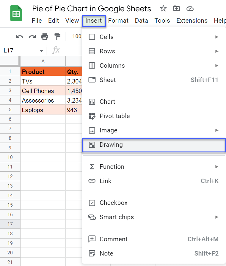
1. Go to the Insert tab and choose “Drawing” from the menu.
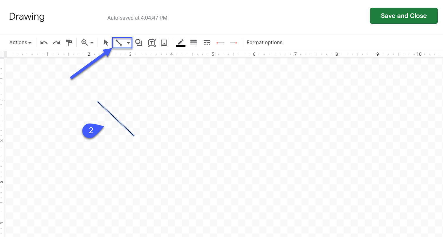
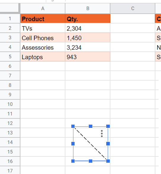
2. Hit the “Line” button and draw a similar line to the one shown in the screenshot below:
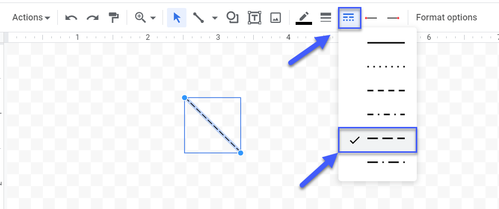
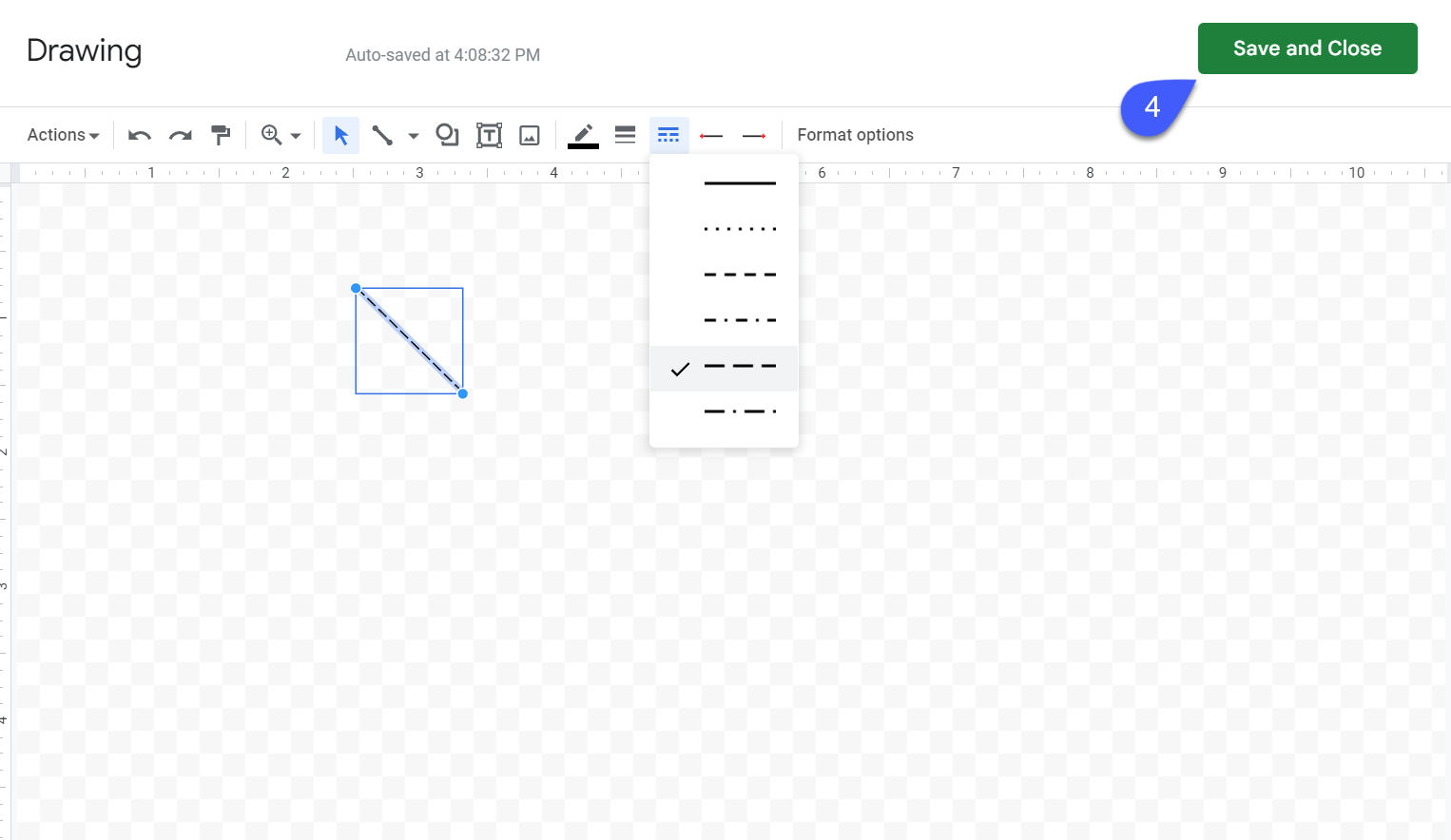
3. Once there, click “Line Dash” and select the fifth option from the top of the drop-down menu.
4. Hit “Save & Close” to create a dashed line.
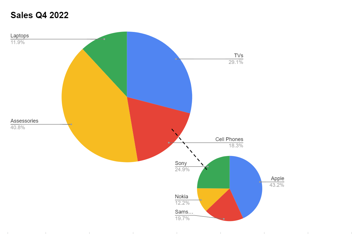
As a result, Google Sheets will generate our dashed line on the spreadsheet.
Now, all you need to do is move it between the primary and secondary pie charts. Having done that, you get your nice-looking pie of pie chart in Google Sheets.