
When working with Excel spreadsheets, you may often need to add additional features to your chart to draw attention to certain indicators and highlight the main purpose of the chart itself.
Excel contains many tools that are easy to master with just a bit of practice. Read on to find out how to add, format, or remove a chart legend in an Excel spreadsheet.
On to the guide!
Prepare Your Data and Chart
To take advantage of Excel’s various functions, you first need to prepare a foundation: the data as well as the chart for your worksheet. If you would like to learn how to do this, we suggest checking out our article How To Create A Column Chart In Excel.
How to Add a Legend to Your Chart in Excel
Using a legend on your spreadsheet will make it much easier to read the data and understand what the chart represents, emphasizing the important points. Follow these simple steps to learn how to accomplish this in a few simple steps:
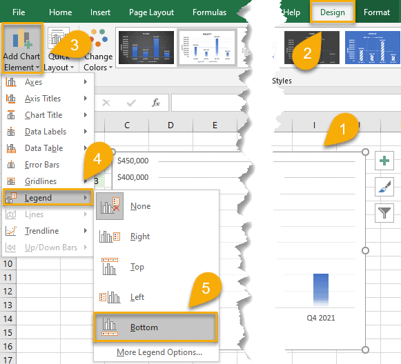
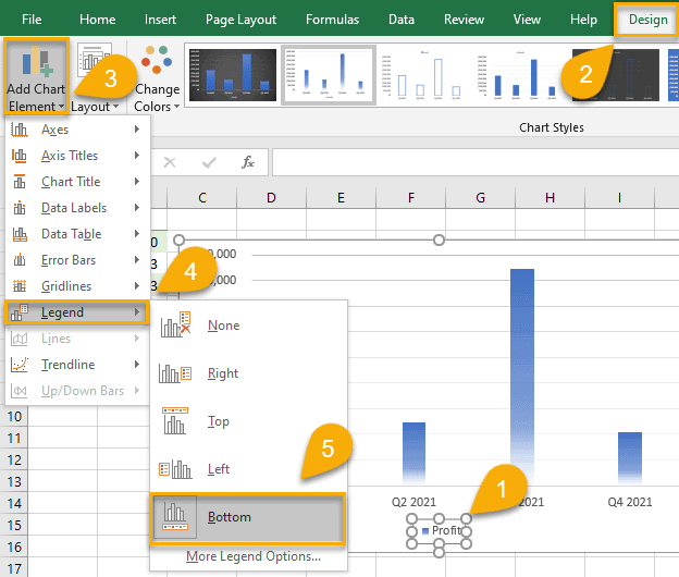
1. Click on your chart.
2. Go to the Design tab.
3. Pick Add Chart Element.
4. Choose Legend.
5. Click Right, Top, Left, or Bottom to set the legend in the position that works best for your chart layout.
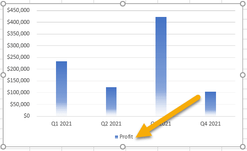
As easy as ABC! Your legend has successfully been added.
How to Format a Legend for Your Chart in Excel
Perhaps you do not want to stick with the default design of the legend, instead making it your own. Excel provides a variety of ways for you to do this. The following step-by-step guide will help you learn your options:
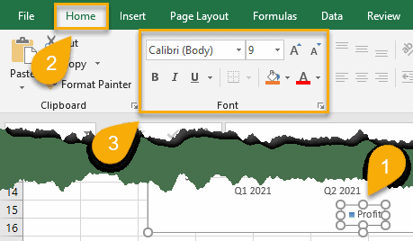
1. Click on the legend for your chart.
2. Select the Home tab.
3. In the Font dialog box, change the font to fit your style. You can choose the font type, color, and size as needed.
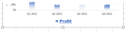
And there you have it. With just a few clicks, you have customized your legend.
How to Remove a Legend from Your Chart in Excel
While having additional information in your chart—such as a legend—generally gives you a better understanding of the data, in some cases, less is best. Thankfully, removing a legend is as easy as adding one. Take a look:
1. Click on the legend.
2. Select the Design tab.
3. Pick the Add Chart Element option.
4. Choose Legend.
5. Click on the type of legend you set before (based on its position), and this will automatically remove it from your Excel chart.
Voila! The unwanted legend has been removed.
Little tips and tricks like these can help you customize your charts and make them stand out from the rest.
