
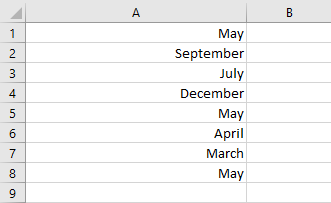
To extract the month from a date in Microsoft Excel, select the cell where you need to enter the month, type the month’s name, and click the month’s name from the list that appears.
There are a number of ways to accomplish this. Let’s take a look at some of the strategies and their procedures to help you pick the one that works best for you!
Method 1: Using the Flash Fill Option
Difficulty: Beginner
Time Estimate: 5 Seconds
1. Click on the cell where you need to enter the month (B1).
2. Start typing the month’s name.
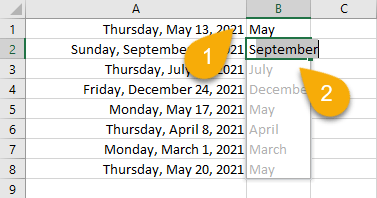
3. Select the name from the list that appears.
This list appears by default, based on the data in the previous column.
Easy-peasy! Just like that, you’ve done it!
Method 2: Using the Format Cells Option
Difficulty: Beginner
Time Estimate: 10 Seconds
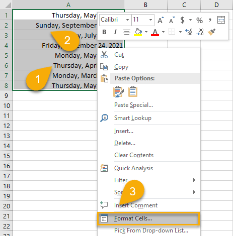
1. Select the cells from where you need to extract the months (A1:A8).
2. Right-click on the selected cells.
3. Choose the Format Cells option.
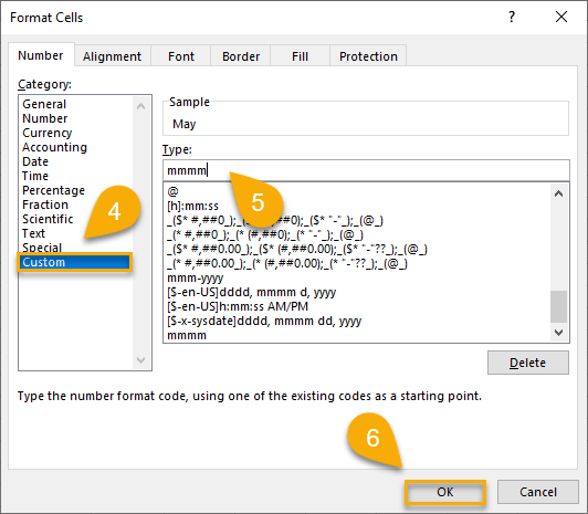
4. In the Number box, pick the Custom category.
5. Type mmm to set the formatting to display the month.
6. Click OK.
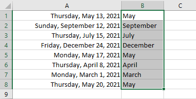
Take a look at the result below!
Method 3: Using the TEXT Formula
Difficulty: Beginner
Time Estimate: 10 Seconds
1. Click on the cell where you want to get the result (B1).
2. Go to the Formula bar and type = TEXT ( A1, “mmmm” ), where A1 is the cell with the date.
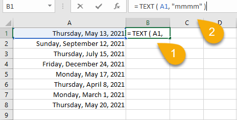
3. Press the Enter key on your keyboard.
4. Drag the cell down to copy the formula for the rest of the list and display all the months in your list.
Easy as ABC!
Method 4: Using the MONTH SWITCH Formula
Difficulty: Beginner
Time Estimate: 25 Seconds
1. Select the cell where you want to show the result (B1).
2. In the Formula bar, type =SWITCH(MONTH(A1), 1,”January”, 2,”February”, 3,”March”, 4,”April”, 5,”May”, 6,”June”, 7,”July”, 8,”August”, 9,”September”, 10,”October”, 11,”November”, 12,”December”). A1 is the cell with the initial date from which you are drawing the month.
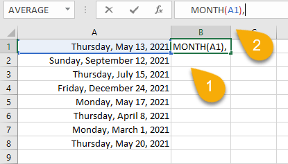
3. Press Enter.
4. To get all the months to show, drag the cell down to copy the formula for the rest of the list.
Piece of cake! Let’s move on to the final formula.
Method 5: Using the MONTH CHOOSE Formula
Difficulty: Beginner
Time Estimate: 25 Seconds
1. Select the cell where you want the month to show.
2. Navigate to the Formula bar and type = CHOOSE(MONTH(A1), “January”, “February”, “March”, “April”, “May”, “June”, “July”, “August”, “September”, “October”, “November”, “December”). Again, A1 is the cell with the date.
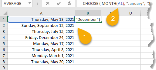
3. Hit the Enter key on your keyboard.
4. Drag the cell down to copy the formula and display all the months.
And there you go!
Dates in Excel FAQs
Do you have questions about using dates in Excel? Let’s take a look at some common questions.
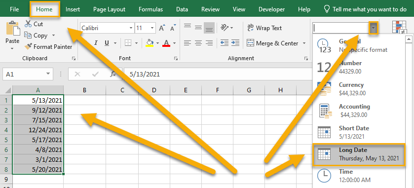
How do I apply the Long Date option?
To apply the Long Date option to your data, select your dates, go to the Home tab, click on the arrow in the Number menu to expand the list, and choose the Long Date option.
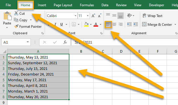
How do I set the alignment for dates?
To set the Alignment for your dates, start by selecting your list of dates, go to the Home tab, and choose the position you like in the Alignment menu (left justified, right justified, centered).
What is the default date format in Excel?
The default date format in Excel is yyyy-mm-dd. This means that the year is represented by four digits, the month by two digits, and the day by two digits. For example, the date January 1, 2020, would be entered as 2020-01-01.
