
As a great tool for operating with large volumes of data, Excel offers a wide range of features for statistical analysis – from the quick analysis tool to built-in add-ins.
And that means that at some point, you’ll inevitably face the need to deal with statistical symbols like x-bar (x̄), y-bar (y̅), p-hat (p̂), and many more.
But how do you actually type them in Excel? Fortunately, you’ve come to the right place.
In this article, you will learn how to type the most common statistical symbols in Excel.
How To Type X-bar (X̅), Y-bar (Y̅), R-bar (R̄), and Z-bar (Z̄)
While using statistical symbols might seem like a daunting task for newbies, in reality, you don’t even need to use functions or complex formulas to pull off the task.
An x-bar and y-bar refer to the arithmetic means of x and y values.
For those looking for a quick solution, just copy and paste those symbols into your worksheet:
- X-bar – X̅ and x̄
- Y-bar – Y̅ and y̅
- R-bar – R̄ and r̄
- Z-bar – Z̄ and z̄
If you’re looking to master the art of working with statistical symbols, here’s how you can create them.
Since this symbol is nowhere to be found on your keyboard, typing it involves a series of simple steps:
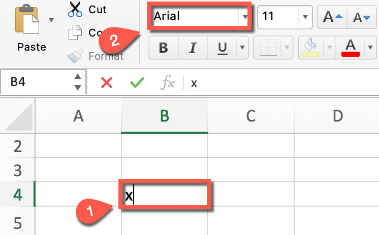
1. Enter “x” into any empty cell – if you want to type a y-bar, enter “y” instead (you get the drill).
2. Set your font to “Arial.”
3. Go to the Insert tab.
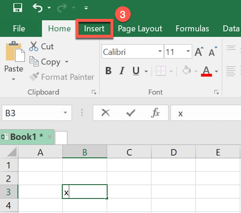
4. In the Symbols group, hit the “Symbol” button.
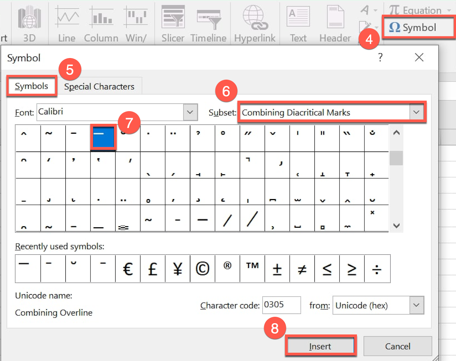
5. In the Symbol dialog box, switch to the Symbols tab.
6. From the Subset drop-down menu, select Combining Diacritical Marks.
7. Pick “Combining Overline” from the list of special characters.
8. Hit “Insert” to close out.
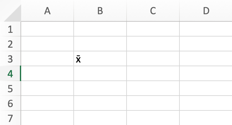
Once there, your x-bar symbol should appear.
If you want to learn more about how to crunch the numbers, here’s how to find X bar.
How to Type X-hat (X̂), P-hat (P̂), K-hat (k̂), Q-hat (Q̂), and D-hat (D̂)
Using a hat with any symbol – be it an x-hat or a p-hat – indicates an estimated value. A quick rule to remember: bars are averages while hats are estimates.
But actually typing any of these statistical symbols in Excel can be a bit tricky. Fortunately, there are multiple ways to work around the issue.
First, for those looking to copy the symbol they’re looking for and take off, here’s the list of them to save you up some time:
- X-hat – X̂ and x̂
- P-hat – P̂ and p̂
- I-hat – Î and î
- G-hat – Ĝ and ĝ
- J-hat – Ĵ and ĵ
- K-hat – K̂ and k̂
- D-bar – D̂ and d̂
For those who wants to stretch their Excel muscles, here’s the process you should follow:
1. Type “p” into any empty cells, for an x-hat, type “x” letter instead – now you catch the drift, right?
2. Set the font to “Arial.”
3. Go to the Insert tab.
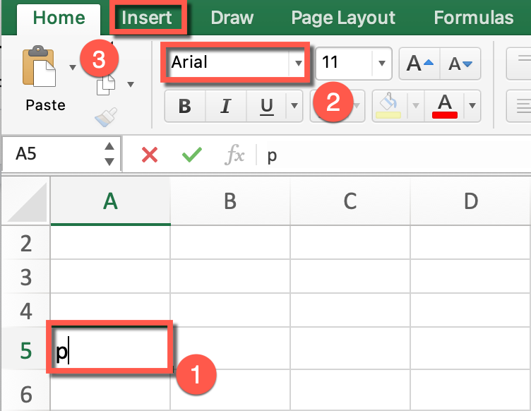
4. In the Symbols group, select the “Symbol” button.
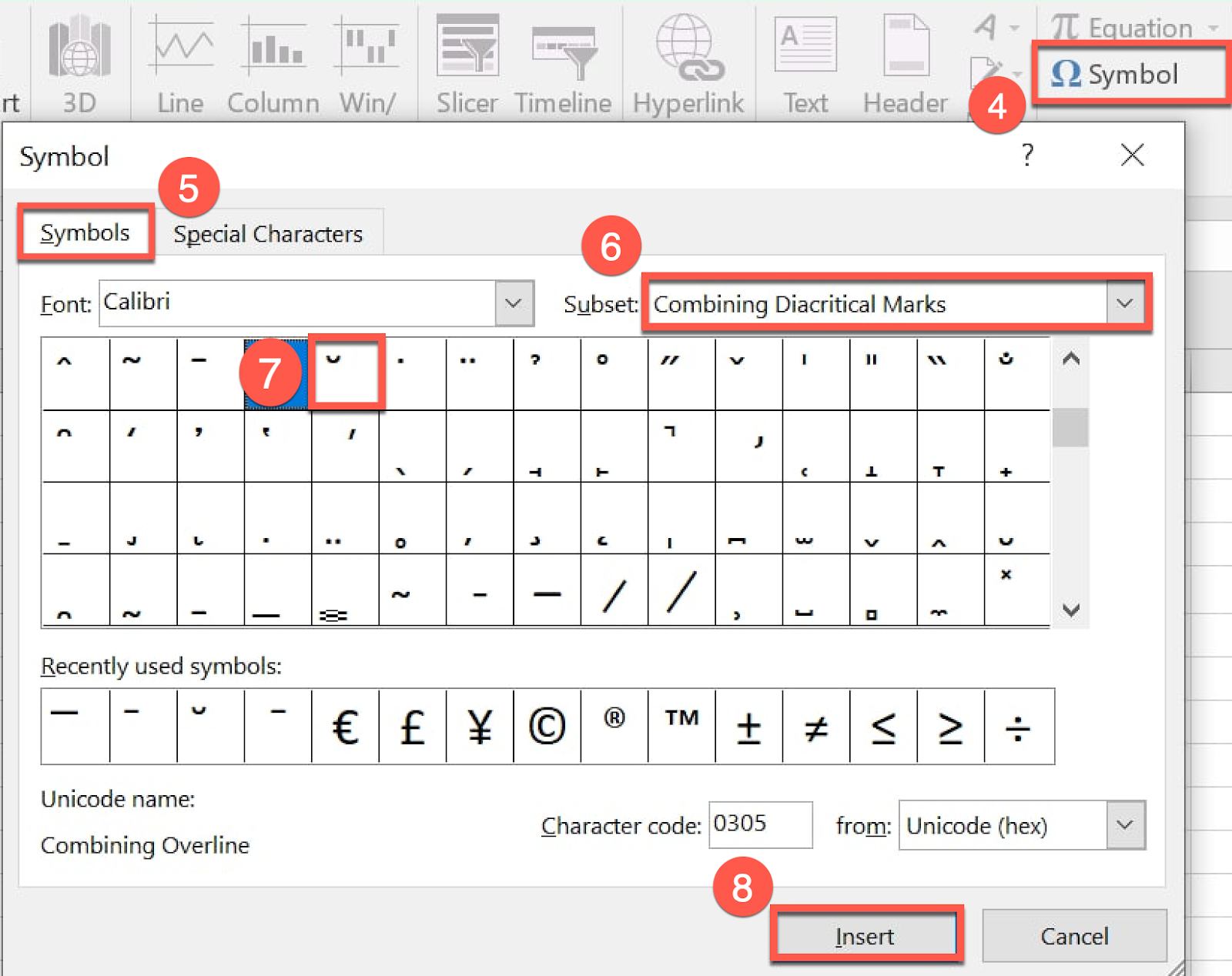
5. In the Symbol dialog box, switch to the Symbols tab.
6. In the Subset drop-down menu, choose Combining Diacritical Marks.
7. Pick the “Combining Overline” symbol (in other words, the hat symbol) from the list of special characters that pops up.
8. Click “Insert.”
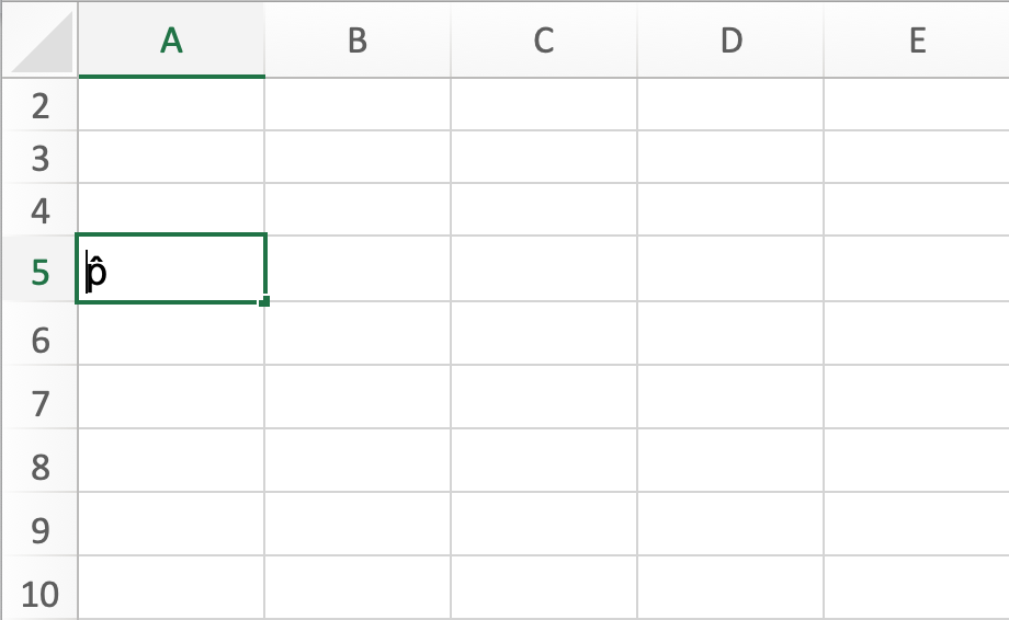
Once you have followed these simple steps, here’s what you should end up with:
While this guide shows you how to use statistical symbols, we’ve barely scratched the surface of what you can do. If you want to learn more about leveraging special characters in your spreadsheets, check out our guide on using the infinity symbol in Excel.
