Sometimes in Excel, you deal with many different numbers in a spreadsheet, each of which may need to be calculated in a certain way. One of the methods that Excel users—experienced and newbies alike—often need to use is a function called “finding X-bar.” This function refers to the arithmetic mean of the elements of a sample.
In this article, you will learn how to find the X-bar easily. All it takes is four simple steps:
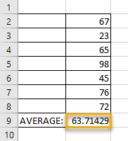
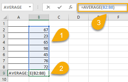
1. Prepare your data.
2. Click on a cell where you need to add the X-bar (here we use B9).
3. On the Formula Bar, type the formula “=AVERAGE(B2:B8),” where “B2:B8” indicates the range of cells containing the numbers you need to find the X-bar.

4. Press the Enter or Tab key.

A piece of cake! Your X-bar has been successfully calculated.
NOTE: If you don’t just need the calculation of the arithmetic mean but also require the symbol of this function, simply copy this: X̅ or x̅. We created a separate guide covering how to type X-bar in Excel – as well as other statistical symbols.
What Is X-Bar and How Is It Used?
The symbol that appears as an “X” with a little dash above it is called X-bar. It refers to the arithmetic mean: namely, the division of the sum of all the numbers in a group by how many are in the group. This tiny symbol is a magic wand when it comes to dealing with a collection of numbers.
The arithmetic mean of the elements in a list is useful for estimating certain statistics. Just divide the sum of the numbers by the quantity of numbers in order to get the results.
Here is the technical formula for finding the X-bar: x̄ = ( Σ xi ) / n, where…
- “X̄” is X-Bar (arithmetic mean),
- “Σ”represents the sum,
- “xi” represents all numbers, and
- “n” represents the quantity of numbers.
It’s that easy!