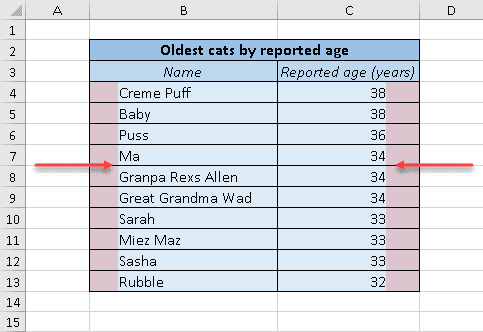
Although Excel is geared toward manipulating numbers—not text—it does make it possible to use some of the features word processors like MS Word offer to make your sheets easier to read.
And indenting is one of them.
This comprehensive guide will show four simple ways to indent text in Excel and help you take another step toward becoming a formatting guru.
Quick Jump
ToggleHow to Indent Cell Data Using a Keyboard Shortcut
This quick-and-dirty method will come in handy for those who prefer using the keyboard.
1. To increase the indent, highlight the cells you want to format (B4:B13).

2. Press the ALT + H + 6 combination.
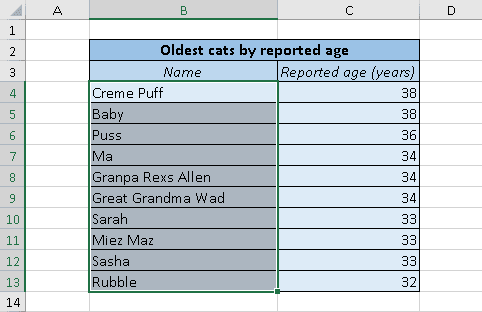
3. To decrease the indent, choose the same cells (B4:B13).
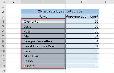
4. Press the ALT + H + 5 combination.

Awesome! We’ve just returned the table to its original look without taking our fingers off the keyboard.
How to Indent Cell Data Using the Ribbon
The Ribbon provides you with quick access to the most common Excel features, allowing you to indent cell contents in just a few clicks.
Here’s how you can do it:
1. Select the cells with the content you want to indent.
2. Click the Home tab.3. In the Alignment group, click the “Increase Indent” button. You can do it multiple times to indent the text as far as you want.
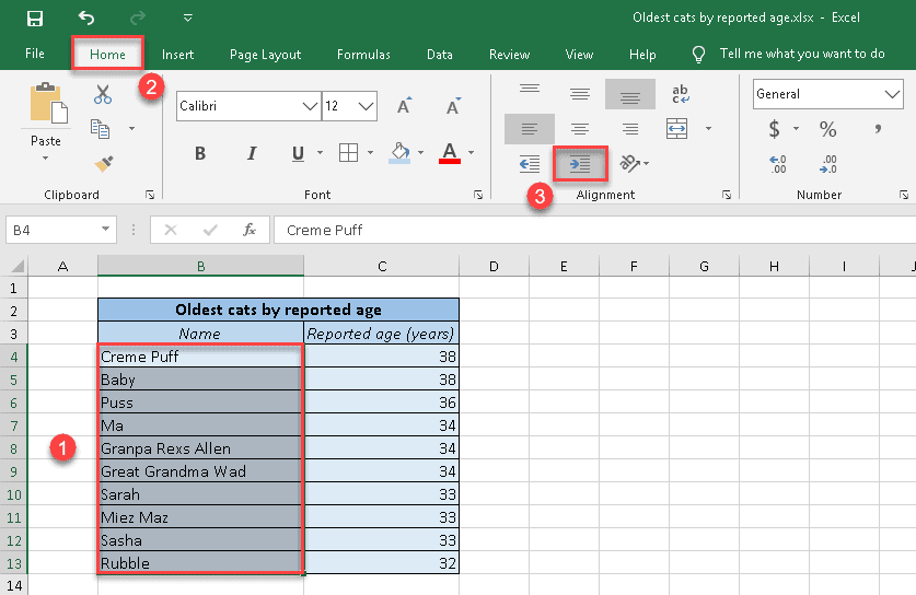
That’s all there is to it, but now let’s deal with the second column that contains numbers. As you can see, they are aligned to the right.
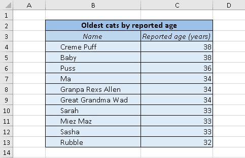
If you try to indent both columns at the same time, the data in column C will automatically become aligned to the left. Text alignment settings in Excel affect indenting in the following ways:
- If the data is left-aligned, it’s indented from the left.
- If the data is right-aligned, it’s indented from the right.
- If the data is centered, it automatically becomes right-aligned and then is indented from the left.
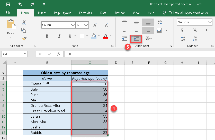
4. So, if you don’t want the numbers to become left-aligned, select them separately.
5. Then click the “Increase Indent” button in the Alignment group (we’ve clicked it three times again).
Now both columns have the same indentation, from either side.
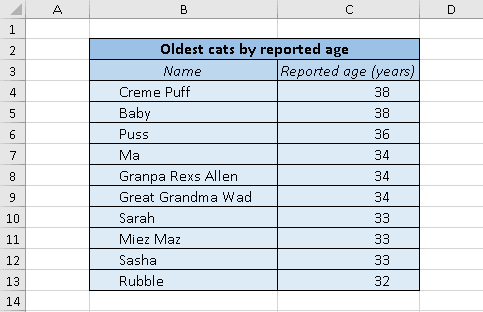
Looks nice! But what would you do if you wanted to decrease or remove the indentation applied to some or all of your worksheet cells?
6. To do that, select the cells where you want to decrease the indentation (we’ve selected the non-adjacent cells by holding down the Ctrl key).
7. In the Alignment group, click the “Decrease Indent” button (we’ve done it three times here as well).
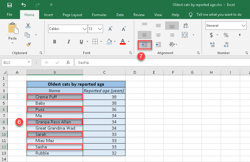
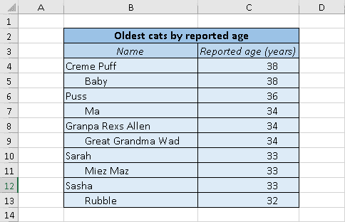
Here is what you get as a result:
How to Indent Cell Data Using the “Format Cells” Dialog Box
This method takes a little bit longer than the others, but it can save you some time when you need to apply several formatting settings at once.
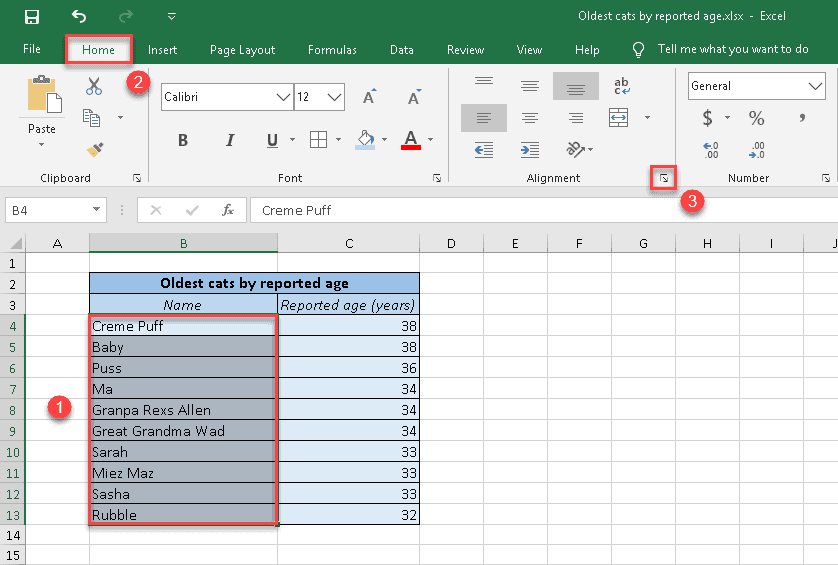
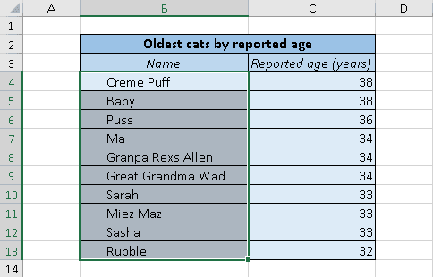
1. Select one or more cells you want to indent (B4:B13).
2. Click the Home tab.
3. In the “Alignment” group, click the “Alignment Setting” dialog box launcher (the small arrow in the bottom right corner).
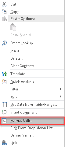
Alternatively, you can press the Ctrl + 1 combination or right-click on the selected cells and choose “Format Cells…” from the drop-down list.
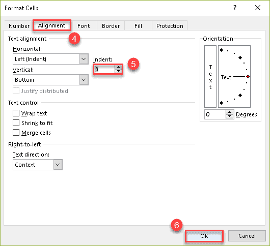
4. In the “Format Cells” dialog box that appears, switch to the Alignment tab.
5. Under the “Text alignment” heading, you can specify the number of characters you want for your indent by typing it manually or using arrows to choose it (in our case, we selected “3”).
6. Click “OK.”
Congratulations! You’re terrific.
How to Indent Lines Within One Cell
Let’s imagine you have a cell whose content is separated with the help of a line break, and you want only one line to be indented.
Bad news: you cannot do it using the methods described above because the indentation will automatically apply to the whole cell.
Good news: you can still get what you want using the good old Spacebar!
Why don’t we start with inserting a line break?
1. Double-click on the cell (we’ll take “B4” as an example) or click once and press the F2 key to enter editing mode.
2. Place the cursor before the word in the text where you want the line break (we’ve chosen the word “Tabby”).
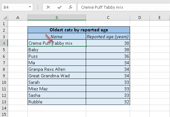
3. Press the Alt + Enter combination (press and hold down the Alt key and then press Enter).
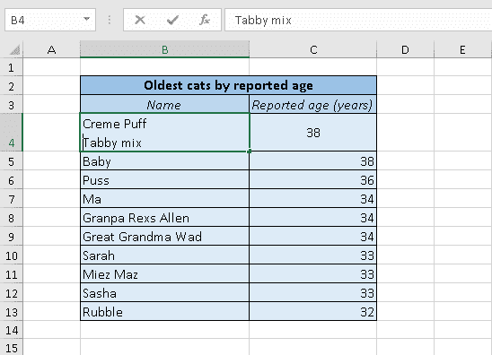
Now that we have two separate lines, let’s adjust the indentation.
4. Place the cursor at the beginning of the line you want to indent (we’ll do it with the second one).
5. Press the Spacebar until you’ve got the desired indentation. Make sure you remember the number of spaces you entered in case you need to repeat it with other lines.
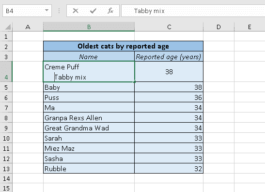
With a little effort, even this clumsy method can bear fruit.
Useful tip: if you want to make your spacing more accurate, you can use one of the monospaced fonts—for example, Courier New.
Why Would I Need to Change Indentation?
By default, any text typed into a cell is aligned to the left while numbers are aligned to the right:
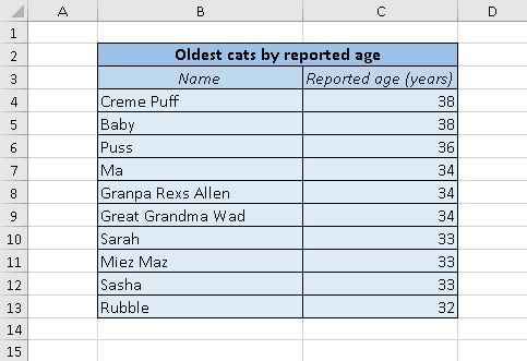
Instead of moving the text or number directly to the right or left edge of the cell, you may want to add some extra space, like when you press the Tab key in Word. However, if you try to do this in Excel, it will simply take you to the next cell on the right.
Fortunately, Excel allows you to achieve the same result by increasing or decreasing the indentation of cell contents.

Yes, you can just press the Spacebar twice, but doing that when you operate with a large number of cells is way too time-consuming.
Moreover, you can get into trouble if you find yourself having to delete all the spaces, or you forget how many of them you used to achieve the desired indent. That’s why using the built-in indentation tools is always a better choice.
Of course, indenting in Excel is not something you need all the time, but this function can serve a number of useful purposes such as:
- Emphasizing the hierarchical structure of a list
- Drawing attention to an important piece of data
- Organizing the data in a more legible way
Now you know everything about indenting in Excel and can easily use it for breathing new life into your spreadsheets!