To pull data from multiple worksheets in Microsoft Excel, first click on the cell where you want the result, then type the formula =Sheet1C3+Sheet2!C3+Sheet3!C3 in the Formula bar, press Enter, and drag the cell down to copy the formula into the following cells.
Let’s go through the process step by step to help you understand it in greater detail!
Quick Jump
Toggle3 Methods to Pull Data from Multiple Worksheets in Excel
Below, we provide three distinct approaches to this task. Choose the method that works best for you.
Method 1: Pulling Data Using a Formula
Difficulty: Beginner
Time Estimate: 2 minutes
1. Go to the primary worksheet where you need the data gathered together.
2. Click on the cell where you want to show the result.
3. In the Formula bar, enter the formula =Monday!C3+Tuesday!C3+Wednesday!C3, where C3 is the cell with the information you need to collect on each worksheet, and Monday/Tuesday/Wednesday are the names of your worksheets with this data.
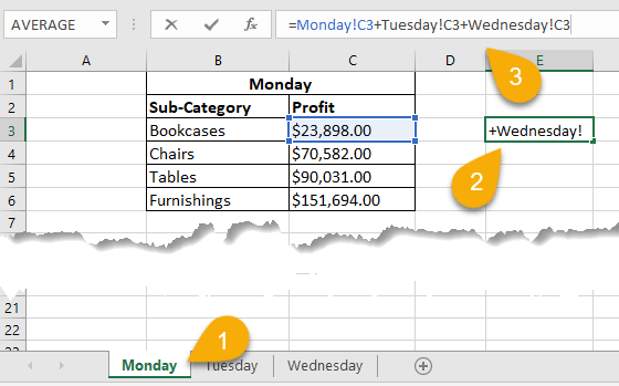
4. Press the Enter key on your keyboard.
5. Right-click on this cell and drag it downward so it copies the formula into the remaining cells.
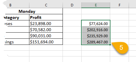
Easy-peasy! Just like that, you’ve summarized all of your data from each worksheet in one place.
Method 2: Pulling Data Using a VBA Code
Difficulty: Advanced
Time Estimate: 6 minutes
1. Navigate to the View tab.
2. Click on the Macros option.
3. Pick View Macros.

4. Under Macro name, type a name for the macro you will create.
5. Click Create.

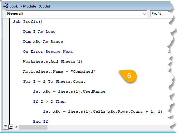
6. Enter this code in the Module:
Sub Profit()
Dim I As Long
Dim xRg As Range
On Error Resume Next
Worksheets.Add Sheets(1)
ActiveSheet.Name = “Combined”
For I = 2 To Sheets.Count
Set xRg = Sheets(1).UsedRange
If I > 2 Then
Set xRg = Sheets(1).Cells(xRg.Rows.Count + 1, 1)
End If
Sheets(I).Activate
ActiveSheet.UsedRange.Copy xRg
Next
End Sub
7. Go to the Run tab.
8. Select Run Sub/UserForm.

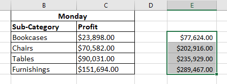
A new worksheet with all the data will now be added to your Excel document.

To summarize everything and create a single table with all of the data, use the procedure above to get the result.
And there you go!
Method 3: Pulling Data Using the Consolidate Function
Difficulty: Beginner
Time Estimate: 5 minutes
1. Click the cell in which the retrieved data should be pasted.
2. Go to the Data menu.
3. Select the Consolidate option.
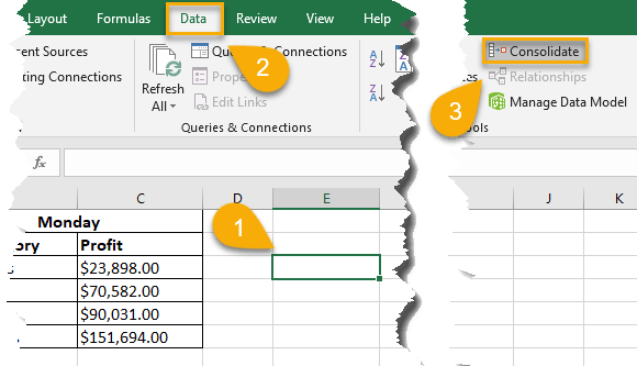
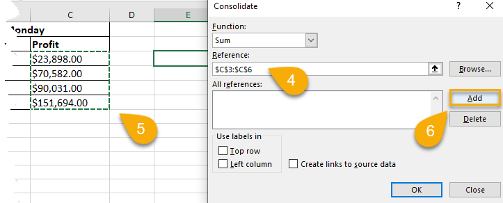
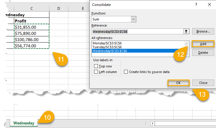
4. In the Consolidate dialog box, navigate to the Reference section.
5. Select the range of the data you need.
6. Hit the Add button.
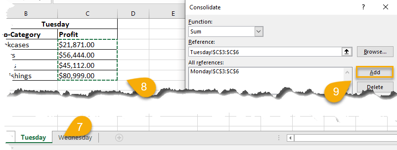
7. Go to the second worksheet.
8. Select the new reference.
9. Click the Add button again.
10. Finally, navigate to the last worksheet.
11. Highlight the data under Reference.
12. Click the Add button again.
13. Press OK.
Voila! The data from all three worksheets has been consolidated onto the first worksheet.

Pulling Data from Multiple Worksheets in Excel FAQs
We’ve compiled a list of solutions to some of the most frequently asked questions about pulling the data from several worksheets in Excel.
What Are the Practical Aspects of Pulling Data from Multiple Worksheets in Excel?
When it comes to managing data in Excel, one of the most important skills you can learn is how to pull data from multiple worksheets. This can be a lifesaver when you need to consolidate information from multiple sources into one place. The advantages of this function include:
- More Organized and Summarized Data: Summarize your data in a single sheet using the techniques outlined above. It may also be more convenient for you to view the data in one place rather than shifting from one worksheet to another.
- Avoid Mistakes: Prevent errors that may occur when you manually summarize data.
Is There a Limit to How Many Worksheets I Can Pull Data From?
No, there is no limit to how many worksheets you can pull data from. However, keep in mind that each additional worksheet will add to the processing time required to retrieve the data. As such, it is generally best to limit the number of worksheets to those that are necessary.
How to Summarize All Values in the Table
We are confident that after following the step-by-step process above, you will be able to obtain all values from all tables. However, you may still wish to compute the total of all the numbers, not just list them.
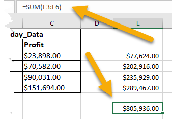
The solution here is easy. Click on the cell where you want to show the total value then type in the Formula bar =SUM(E3:E6), where E3:E6 is the range with your values, and press Enter.
