
To ignore zeros when averaging cells in Google Sheets, use the following custom formula: “=AVERAGEIF(B1:B5, “<>0”)” where “B1:B5” is your cell data range.
In this article, we’re going to break down, step-by-step, how you can apply this custom formula to your data.
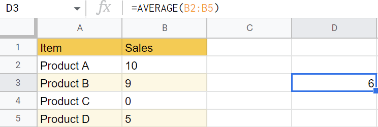
Why the AVERAGE Function Doesn’t Cut It
Well, the answer is simple.
When you apply the AVERAGE function in Google Sheets, you count in zeros, which may end up skewing your data depending on your goals.
Here’s how it works in practice:
That’s why whenever you need to skip zeros completely, you need to deploy the AVERAGEIF function that allows you to apply the IF statements blocking out zero values when averaging your values.
And the beauty of this method is that it’s ridiculously easy to use. Just follow the steps below.
How to Exclude Zeros When Averaging Cell Values
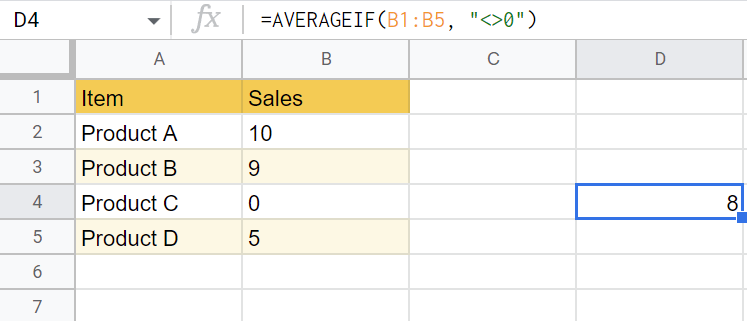
As mentioned above, to exclude zero values when averaging in Google Sheets, here’s how you can deploy the AVERAGEIF function.
- Select any empty cell where you want Google Sheets to return the function output.
- Type “=AVERAGEIF(B1:B5, “<>0”)” into the Formula bar and type Enter.
Once there, you get the result without accounting for the zero values within the data range you picked.
If you’re curious about how the customized version of the AVERAGEIF function works, here’s the breakdown:
- By design, the AVERAGEIF function returns the average value depending on criteria. Alternatively, we could have used the AVERAGEIFS function to achieve the same outcome.
- “B1:B5” is the cell range the function runs through and applies to the conditions specified in the second part of AVERAGEIF.
- “<>0” is the second part of the equation where we use the Google Sheets Does Not Equal operator to signify that we don’t want to count in zero values when averaging the values within the specified cell range.
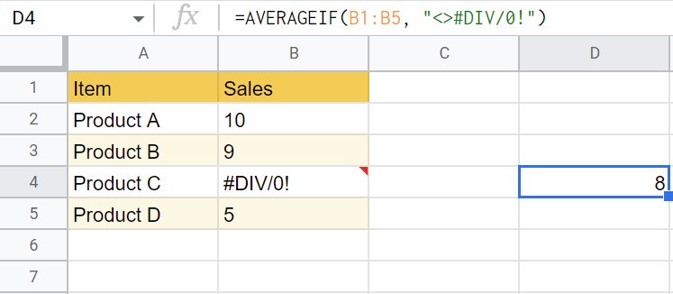
How to Ignore the “#DIV/0!” Error When Averaging Values
To ignore the divide by zero error (#DIV/0!) when averaging values in Google Sheets, use the following function:
=AVERAGEIF(B1:B5, “<>#DIV/0!”)
This modification of the AVERAGEIF function ignores all the instances of the #DIV/0 error in your data set, helping you complete the averaging process without triggering an error.
Now, over to you. By following these simple steps, you can easily average values without skewing your results when you have a bunch of zero values in your data set.
