
Checklists are a great way to keep track of tasks and responsibilities. They can help you stay organized and ensure that all the necessary steps are completed. Google Sheets is a versatile tool that can be used for various purposes, including creating checklists.
This article will show you how to create a checklist in Google Sheets, both in a web browser and on the Google Sheets app.
How to Сreate a Checklist in Google Sheets (Web)
To create a checklist in Google Sheets, you’ll need to start with some basic details.
We’ll begin by creating a simple checklist with two columns: one for the tasks themselves and one for the status of each task.
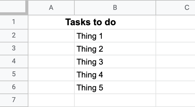
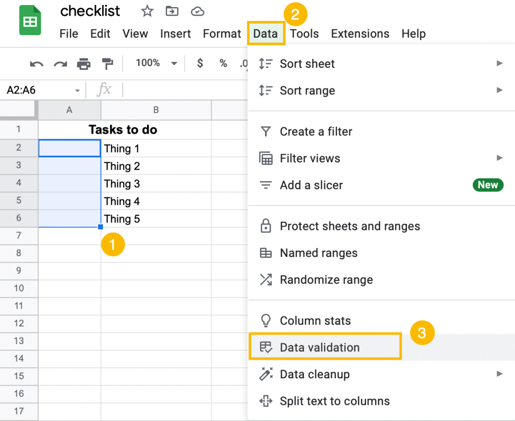
1. Select the cells you want to format as the checklist, showing the status of each task (A2:A6).
2. In the main menu, click Data and select Data validation from the list.
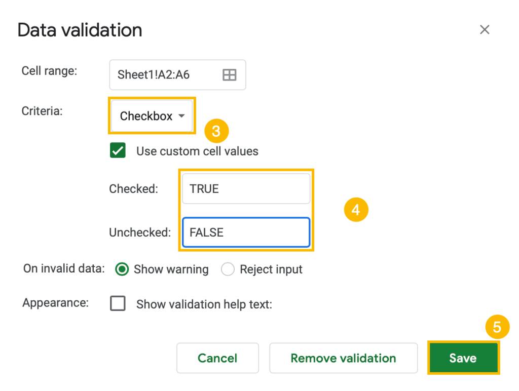
3. In the Data validation box, under the Criteria section, choose Checkbox.
4. Check the box beside the Use custom cell values option. Enter TRUE in the first cell (Checked) and FALSE in the second cell (Unchecked).
5. Click Save to apply your changes.
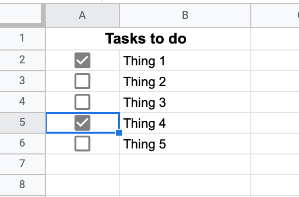
That’s it. Easy-peasy! Your checklist is done. To turn a dull checklist into a design element, consider using Google Sheets emojis and conditional formatting.
How to Create a Checklist in Google Sheets (Mobile App)
Creating a checklist is even easier in the Google Sheets mobile app. Open the app and let’s take a look!
We will use the same example data.
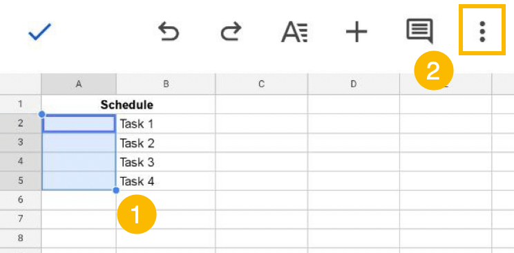
1. Highlight the cells where you want your checklist (A2:A5).
2. Click on the three dots in the top right corner of the screen.
3. Go to Data validation.
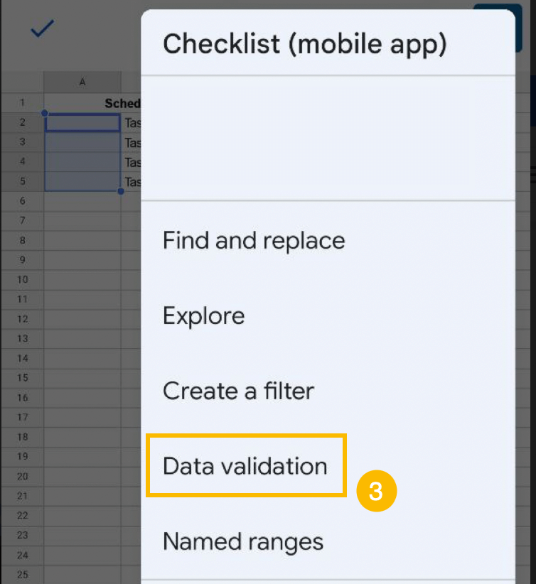
The Data validation box will appear.
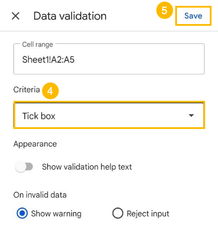
4. Under Criteria, select Tick box from the menu that appears.
5. When finished, tap the Save button in the top-right corner of the screen.
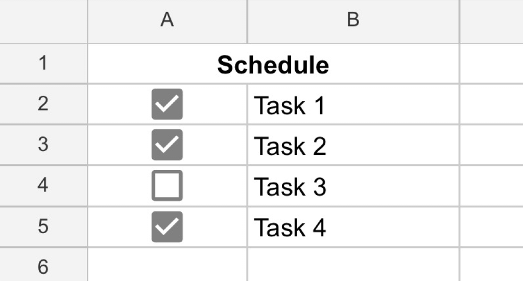
Your checklist is done! Now you can quickly tick or untick to show whether or not each task has been completed.
BONUS TIP: How to Apply Conditional Formatting to a Checklist in Google Sheets
One very helpful option is Google Sheets is the use of conditional formatting to highlight the status of your tasks. This visualization tool can help you see at a glance what tasks still need to be done.
To set this up, follow the steps below.
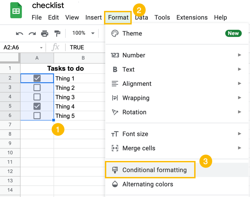
1. Select the cells containing the checkboxes (A2:A6).
2. Navigate to Format in the main menu.
3. Go to Conditional formatting.
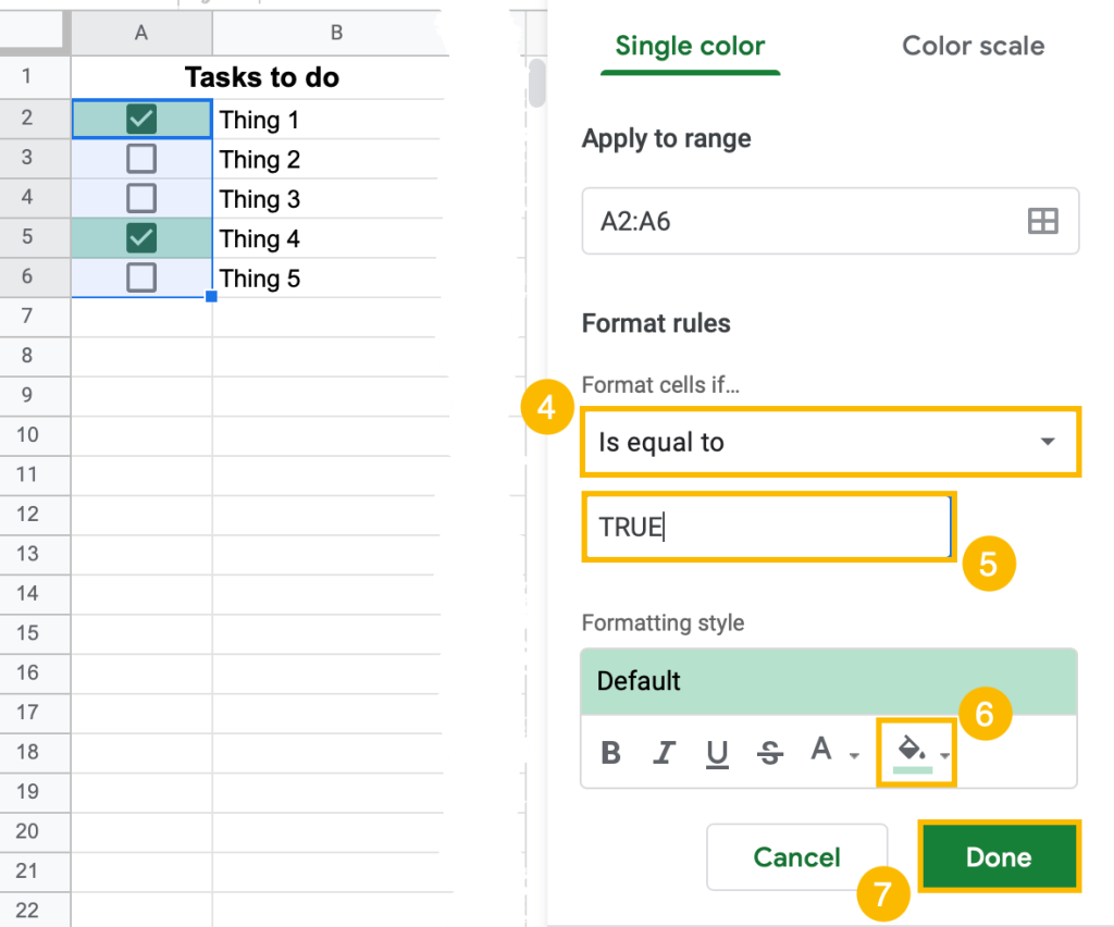
4. In the Format cells if drop-down menu, select Is equal to…
5. Under the Format cells if box, enter “TRUE.”
6. Select the Fill color box to change the color of the cell.
7. Click the Done button.
To highlight other boxes in a different color:
8. Click Add another rule.
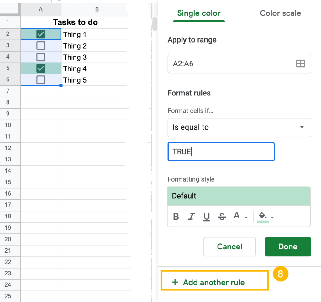
Follow the same steps as you did before:
9. Under the Format cells if… box, enter FALSE.
10. To apply another color to these cells, go to the Fill color box and select the color you want.
11. Save your changes by clicking the Done button.
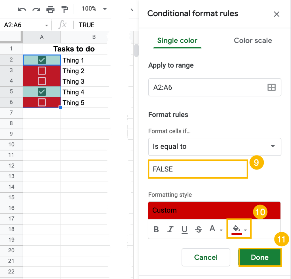
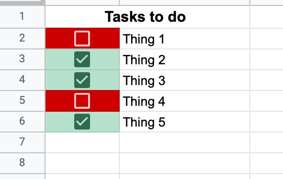
Highlighted tasks make it easy to see what still needs to be done.
Using checklists in conjunction with drop-down lists, you can quickly create a simple yet powerful project management tool (if you want to learn more, here’s our how-to guide on how to create a drop-down list in Google Sheets).
