When you’re working with a team, you will very likely need to share your spreadsheets with others at one point or another. Google Sheets offers many tools that help you streamline your projects, making it much easier to collaborate with teammates.
One such tool is the drop-down list.
Say, for example, that you have multiple projects going on at the same time. You might create a Kanban board to keep track of all your tasks. Having a drop-down list could make it quite simple to update the status of each as needed.
Quick Jump
ToggleHow to Create a Drop-down List
Let’s dive into creating our very own drop-down list. To start off with, open Google Sheets and either select an existing spreadsheet or make a new one.
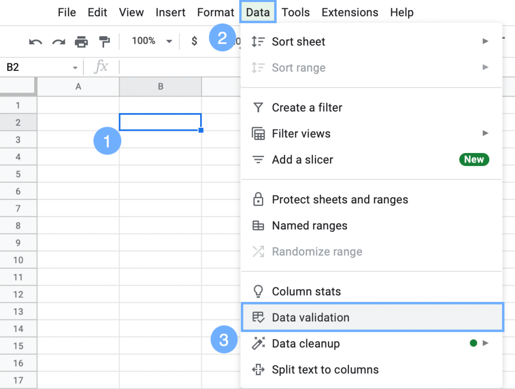
1. Select the cell (B2) where you wish to create your drop-down list.
2. Click Data in the menu along the top.
3. Go to Data validation.
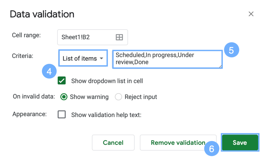
The Data validation window will appear.
4. In the Criteria box, select List of items.
5. In the box, enter the items for your list, separating each one with a comma.
6. Click Save.
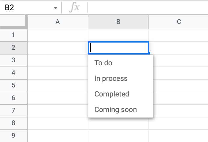
It’s that easy! Your drop-down box is ready to go.
How to Color a Drop-down List
For better visualization, you can add colors to the items in the drop-down list. It makes it handy to see the status of each item at a glance.
1. Select Format.
2. Open the Conditional formatting menu.
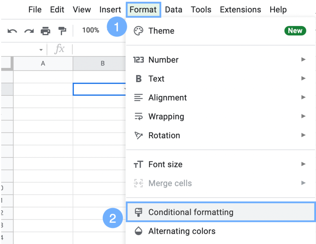
To apply color to each item in your drop-down list, follow these steps:
3. Switch to the Single color tab in the task pane window.
4. Under Apply to range, insert the cell where you made the drop-down list (B2).
5. Under the Format cells if box, select Text is exactly.
6. In the text box immediately below that, enter the text you want to apply to a particular color.
7. Select Fill color to attach a color to that option.
8. Click the Done button when finished.
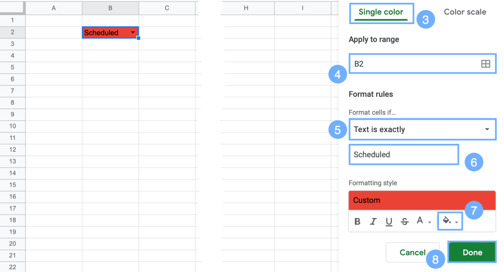
To apply color to the rest of the options in your list, stay in the same window.
Choose Add another rule.
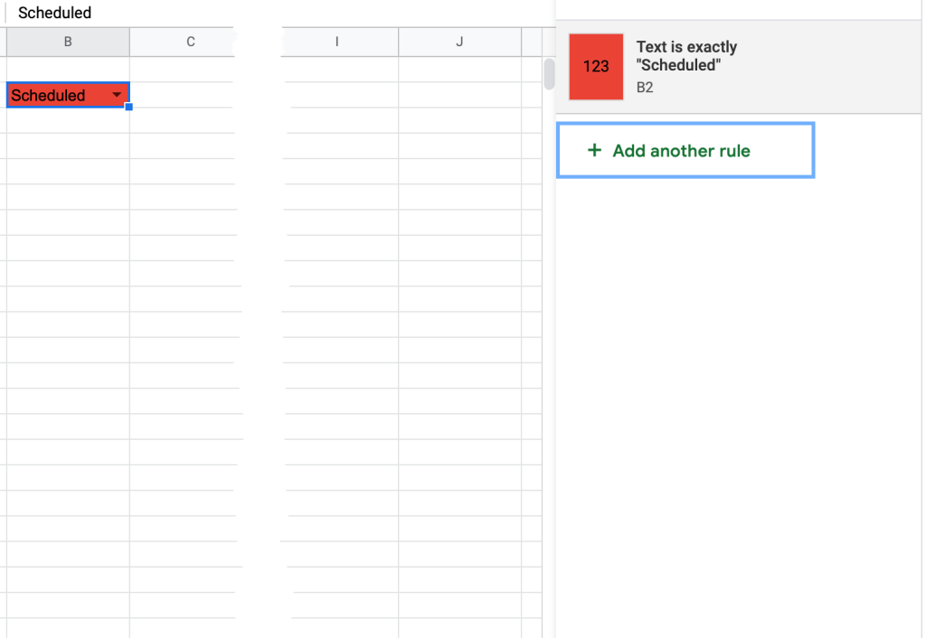
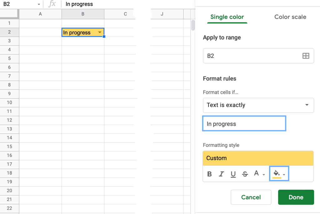
Repeat the steps from before to add color to every item on the list.
If you need to add this drop-down list to other cells, either use the fill handle icon to copy it into the cells directly below it or use copy (Ctrl+C) and paste (Ctrl+V) to add it to another column as required.
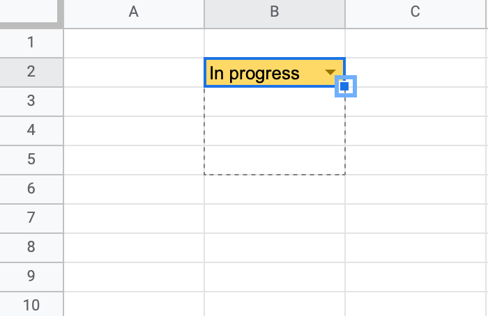
Now your drop-down list is done.
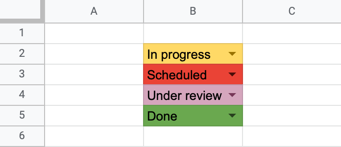
How to Remove a Drop-down List
If you no longer need the drop-down list or simply want to delete it from the cell, don’t worry—that’s easy enough to accomplish. Follow these steps to remove your drop-down list:
1. Select the cell with the unwanted drop-down list (D5).
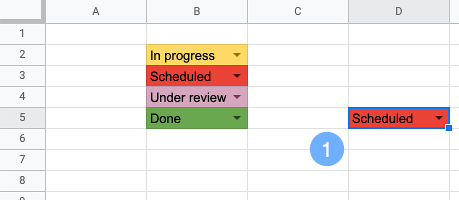
2. Go to Data and choose Data validation.
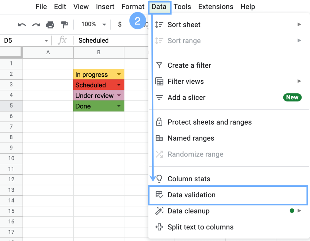
3. Under Cell range, make sure you select the correct cell (D5).
4. Click the Remove validation box.
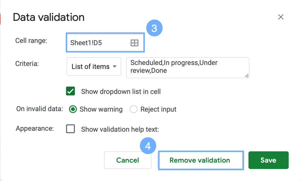
Voila! The drop-down list has been removed.
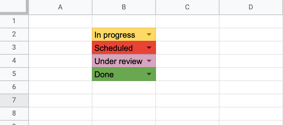
How to Remove the Down Arrow from the Drop-down List
When you create a drop-down list in Google Sheets, the list will automatically show a down arrow on the right side of the cell, indicating that you can select the cell to see a drop-down list.
However, if you would rather not have the arrow showing, it is possible to remove it:
1. Select the cell (or cells) where you want to remove the down arrow (B2).
2. Go to Data.
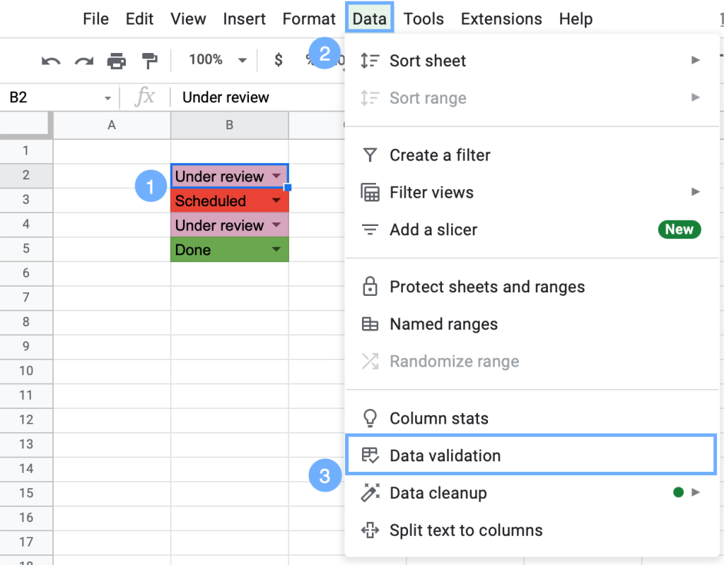
3. Navigate to Data validation.
4. Uncheck the Show dropdown list in cell box.
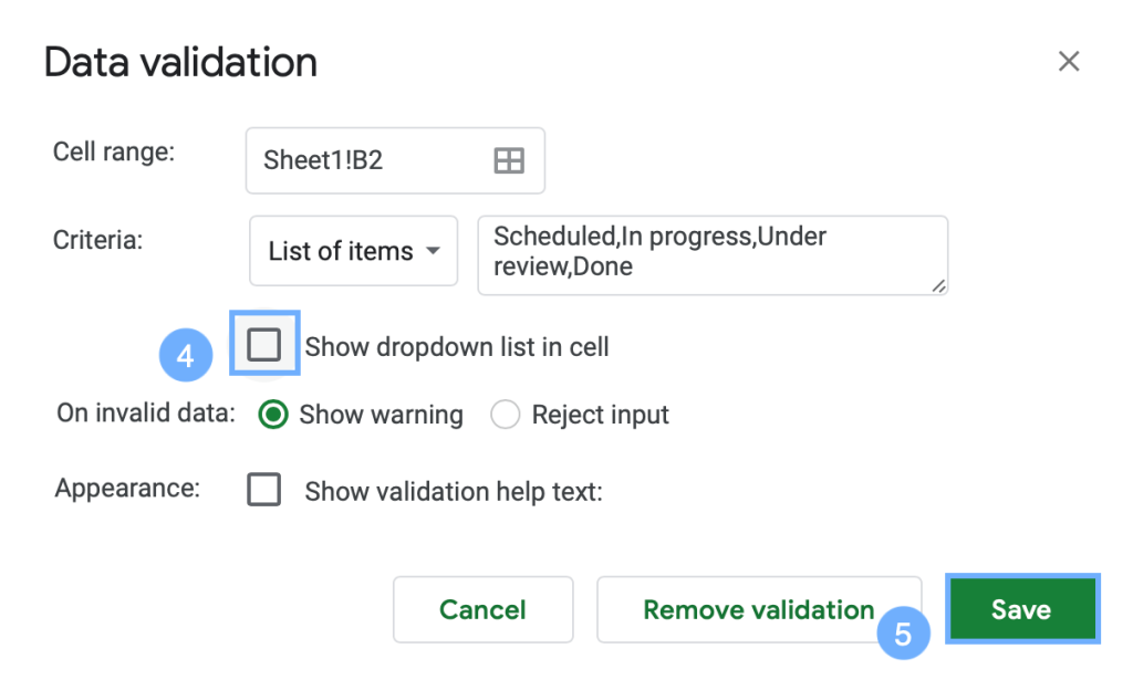
5. Click the Save button.
The cell will no longer display the drop-down list if you click on it once. However, you can either double click the cell to reveal the drop-down list or just type the text for that cell manually. The color coding you have established for the list will still apply.
Use drop-down lists to improve your documents and make life easier for yourself. Plus, you just might impress your colleagues with your Excel skills!