To use conditional formatting with a checkbox in Google Sheets, highlight your cell range, navigate to the Format menu, pick Conditional formatting, select Custom formula is under Format cells if…, type the formula =$B$1=TRUE, choose the cell color, and hit Done.
To ensure you don’t miss anything important about this topic, read through the following article to learn how to use conditional formatting with a checkbox in Google Sheets!
How Does Conditional Formatting with a Checkbox Work?
Conditional formatting with a checkbox works by setting certain conditions or criteria which will change the formatting of the box. Whenever one of these conditions is met, the formatting will be applied to the cells with that condition in place.
For example, you could set a conditional formatting rule that says if a cell contains a checkbox and it is checked, then the background color of that cell should turn yellow.
Conditional formatting can be useful for hiding or highlighting certain cells in a sheet. You could use conditional formatting to hide cells that are unchecked or to highlight cells that are checked. This can help you focus on the most important data in a sheet.
How to Change Cell Color Based on a Checkbox
Use the detailed step-by-step guide and illustrations below to change cell color based on a checkbox in seconds:
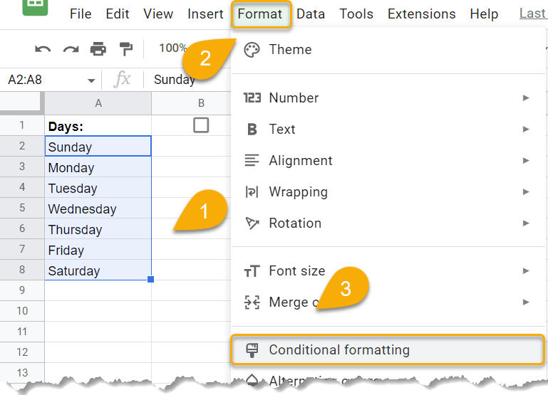
- Select the cells whose formatting you want to change using the conditional formatting rules.
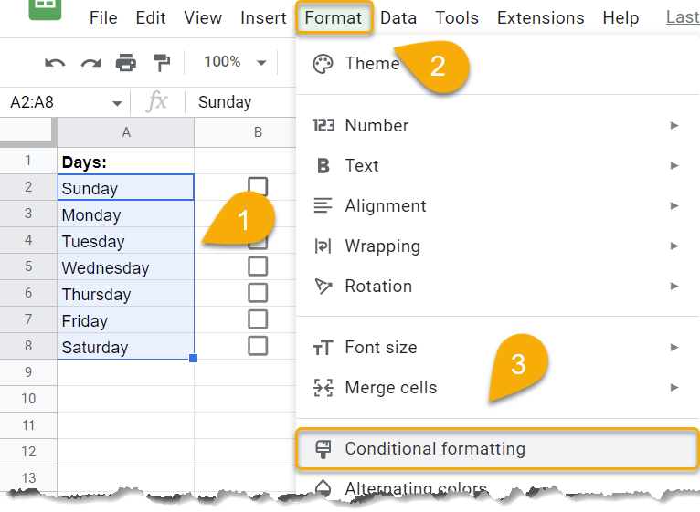
- Go to the Format menu.
- Click on the Conditional formatting option.
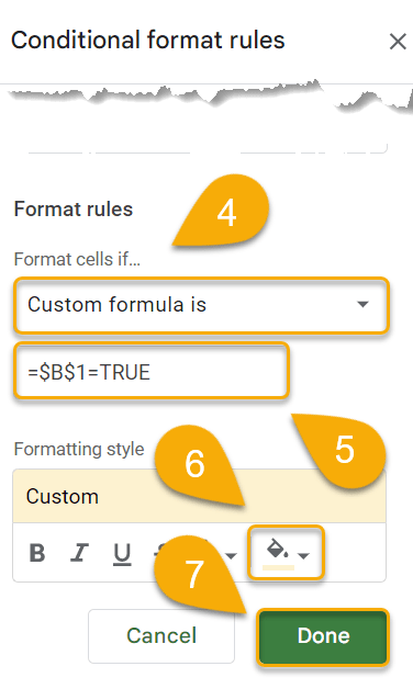
At this point, you will see the Conditional format rules box where you must set the rules that will trigger the formatting changes.
- Under Format cells if…, select Custom formula is.
- Enter the formula =$B$1=TRUE, where B1 is the cell with a checkbox.
- Pick the cell color you like.
- Lastly, press the Done button.
Just like that, it’s done! Let’s take a look at how it works.
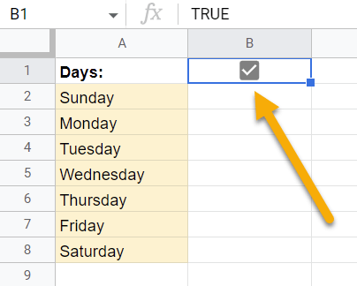
Checking the checkbox will activate the condition and change the color of the cells.
How to Apply Conditional Formatting If Multiple Checkboxes Are Ticked
The above method applies changes to multiple cells based on the condition of one cell. If you want cells to change individually, check out the steps below:
- Highlight the data range.
- Navigate to the Format menu.
- Pick Conditional formatting.
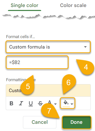
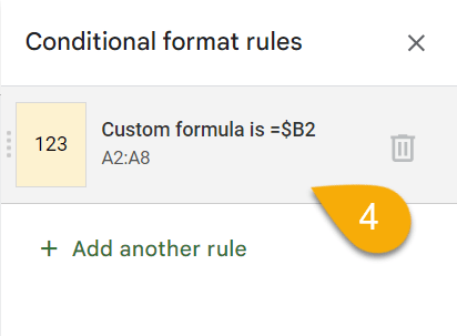
- Under Format cells if…, choose the Custom formula is option.
- Type the formula =$B2. The dollar sign locks the formula to the B column, which is the column with the checkboxes.
- Next, select the cell color you want for the cells when the checkbox is marked.
- Press the Done button.
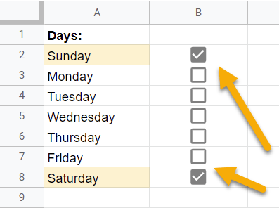
Voila! You can now selectively click on different checkboxes, and the color will change automatically.
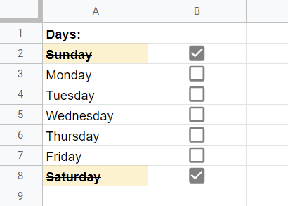
How to Bold, Italicize, Underline, or Strikethrough a Cell Based on Whether a Checkbox is Ticked
Conditional formatting can also affect the formatting style of the text in the cell. To do this, follow the steps described above and then do the following:
- Select your data.
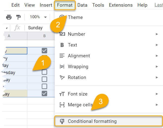
- Go to the Format menu.
- Click on the Conditional formatting option.
- Select the conditional format rule you have already created.
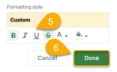
- Choose the Formatting style options you need.
- Lastly, press Done.
Easy as ABC! Your cell’s contents will change as you have directed it. You can see the result below.