
Does your spreadsheet contain a lot of datasets? If so, column or header rows can prove quite vital to your document as they label the contents of each column or row.
If you were to scroll far enough down or to the right, you could lose sight of that valuable line telling you what each column or row represents. You could end up wasting precious time scrolling up and down or back and forth in order to keep track of everything, especially when you want to expand all columns.
Thankfully, Google Sheets gives you the opportunity to ensure that line always remains visible.
Let’s dive into the process of how to freeze one—or multiple—rows or columns in Google Sheets.
How to Freeze One or Multiple Rows in Google Sheets
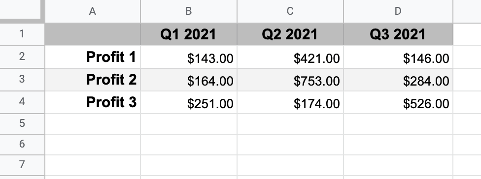
Say you have a header row for your data, and you need to freeze it so it won’t disappear when you scroll down the page. There are two ways to lock it in place.
Method #1
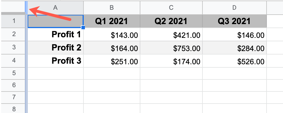
1. Go to the top-left corner part of the sheet, to the left of the default column headers (letters) and above the default row headers (numbers).
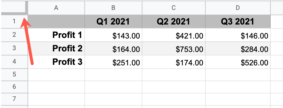
2. Drag the bottom line of that box below the first row.
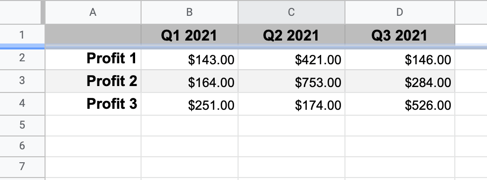
That’s it! The header row is now frozen. You can scroll down to check and make sure it doesn’t disappear.
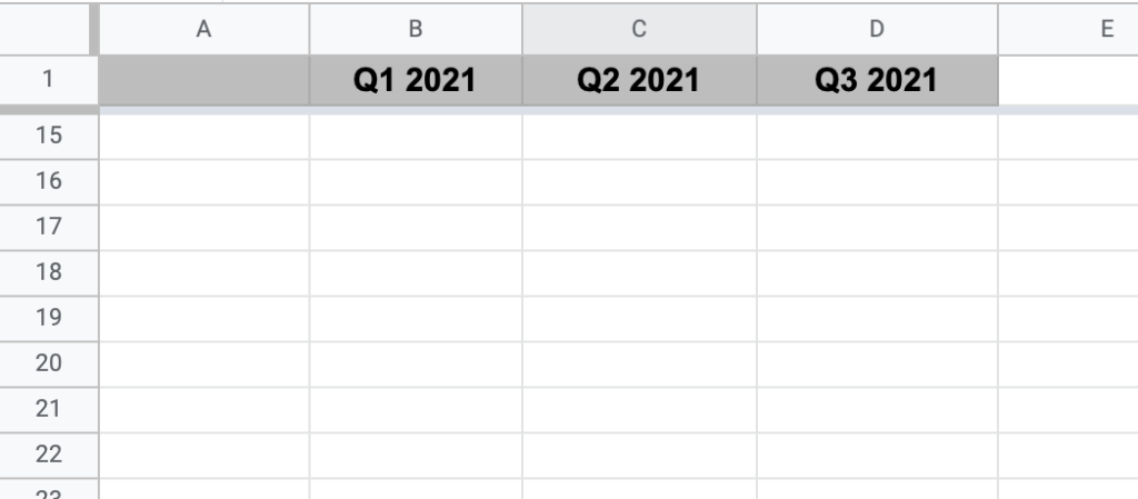
We scrolled down, but as you can see, the first row is still visible. Follow the same process to unfreeze rows.
Note: If you have multiple rows that you need to freeze, just drag and drop the gray “freeze” line after these rows.
Method #2
Alternatively, here’s the second method you can use to lock one row or freeze multiple rows in Google Sheets.
You can also freeze rows using the menu. Here are the steps to do this:
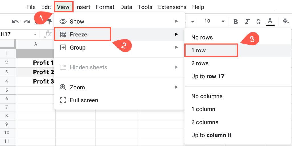
1. Go to the View option in the menu.
2. Select Freeze.
3. From the menu, select 1 row.
Easy-peasy—the top row is now frozen.
You can also select 2 rows if you need to freeze the top two rows. If you need to freeze more than two rows, continue on.
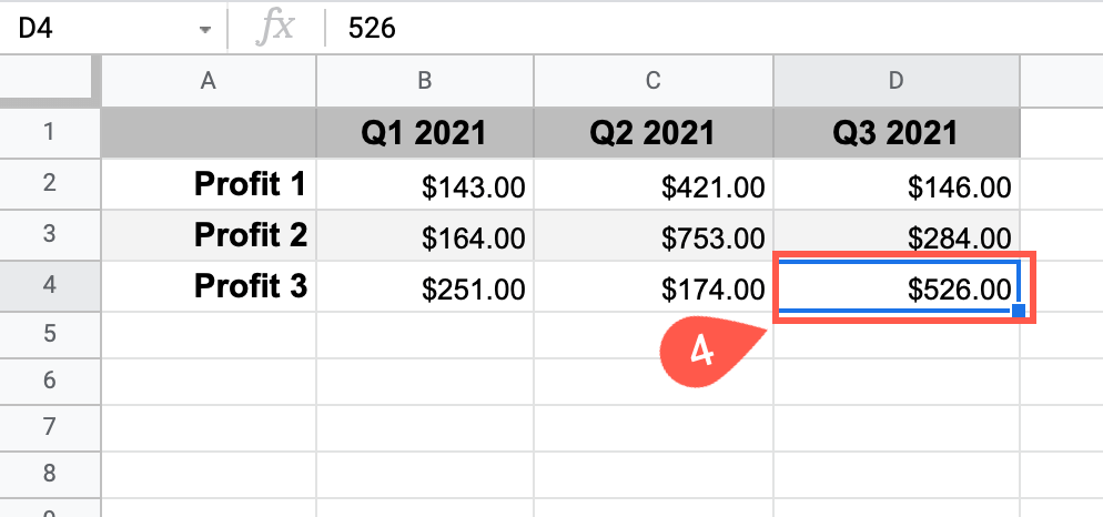
4. Click on any cell in the row to which you want to freeze (in this example, D4).
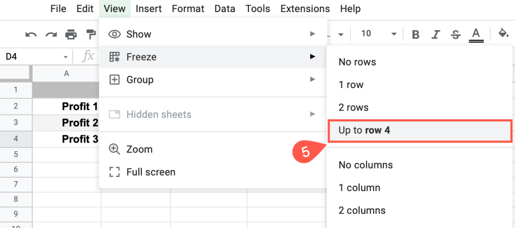
To freeze multiple rows simultaneously, follow the same steps described above: View > Freeze. However, at this point you will select a different option.
5. Select Up to row 4. The specified row is determined by which cell you have selected.
Use whichever method is easiest for you.
How to Freeze One or Multiple Columns in Google Sheets
Freezing columns is just as simple as freezing rows.
1. Go to the top-left corner part of the sheet, to the left of the default column headers (letters) and above the default row headers (numbers).
2. Drag the right border of the corner box to the right edge of the column you want to freeze.
It’s as easy as that! In our example, columns A:C are frozen.
The other option to freeze columns is to use the menu. Follow these simple steps to freeze one or more columns simultaneously as needed for your worksheet:
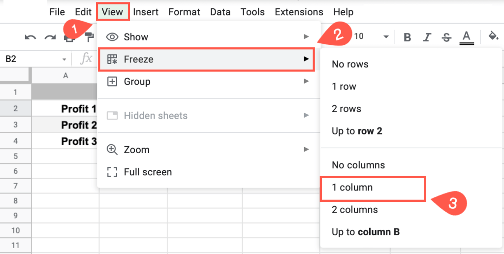
1. Go to the View tab.
2. Choose the Freeze option.
3. Select 1 column or 2 columns.
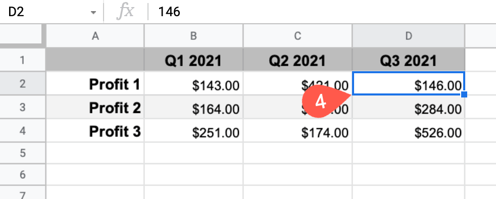
If you are working with more than 2 columns, do this instead:
4. Click on any cell in the furthermost column that you want to freeze (in our example, D2).
Go to View > Freeze.
5. Choose the option Up to column D.
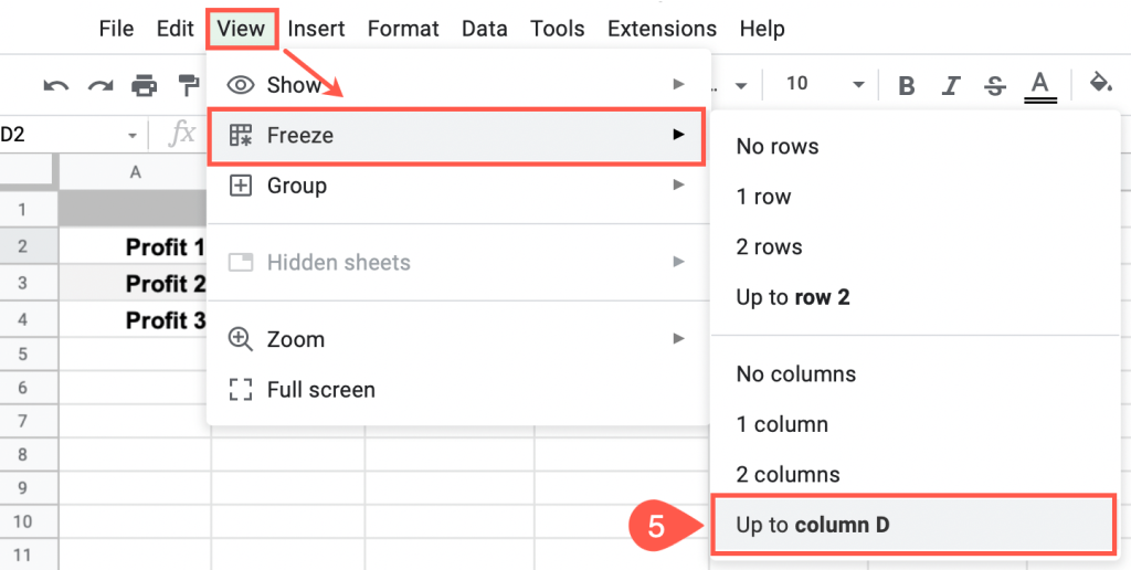
Just like that, your columns are frozen. Select “No columns” to unfreeze columns. The same technique can be used in the Google Sheets mobile app.
You can see that freezing rows and columns in Google Sheets is pretty easy; you don’t need special knowledge or secret tricks. Choose the way that works best for yourself and take advantage of the tools Google Sheets offers to make your life easier.
FAQs
What Does It Mean to Freeze a Row or Column in Google Sheets?
You can freeze a row or column in Google Sheets so that it is always visible, even when you navigate your spreadsheet. Frozen rows and columns are divided by a horizontal gray line.
Why May We Want to Freeze Rows and Columns Using Google Sheets?
Here we give you a few examples in what conditions it is most advisable to freeze rows and columns:
- When you want to keep headers locked in place to define necessary rows or columns with information
- When you want to compare one type of data to another kind throughout your tables
- If you want to keep in mind the critical points when scrolling through data in the spreadsheet.
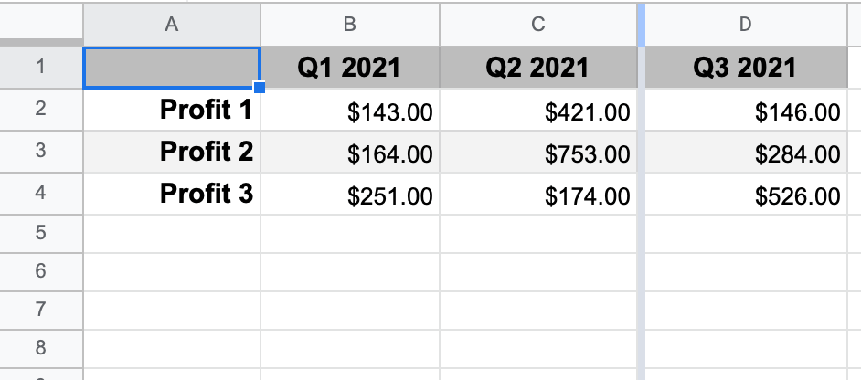
So, imagine you are the owner of a chain of grocery shops “Around the corner.” You keep the records of grocery`s profits/losses in Google Sheets to keep an eye on how your business is developing from quarter to quarter.
In addition, you want to compare the profitability and performance of stores from month to month, observe which store brings the most profit in each reporting period and how financial indicators change.
But it’s so easy to get lost in these numbers and data! Also, if you scroll right or down, the header name and data disappear. And in this case, freezing rows and columns will be more useful than ever. Below we will show how to do this using the Menu bar and Shortcuts.
How Can I Freeze the Top Two Rows in Google Sheets?
If you want to freeze the top two rows in Google Sheets, click the View tab and select “2 Rows.” This will keep them in place while you scroll down the sheet. If you’re looking for more customization options, there are Google Sheets add-ons that allow for more flexibility.
Is There a Way to Freeze Panes in Google Sheet?
Use one of the methods described above to freeze one or panes in Google Sheets rows and/or columns. You can use the menu, keyboard shortcuts, or simply drag the corner box in Google Sheet.
